![Woody Calculus introduction to differential-equation mixing problems, showing a perfectly stirred saltwater tank with inflow and outflow. The governing model is Q′(t) = c_in r_in − [Q(t)/V(t)]r_out. Equal flow rates produce constant volume, while unequal flow rates produce changing volume.](https://k3p6r8v3.delivery.rocketcdn.me/wp-content/uploads/2026/08/Mixing_Problems_Slide_01.png)

Learn how to model and solve differential-equation mixing problems with rate in minus rate out. Work through constant-volume, draining-tank, and overflow examples, then practice the complete seven-step method.
Learn how to model and solve differential-equation mixing problems with rate in minus rate out. Work through constant-volume, draining-tank, and overflow examples, then practice the complete seven-step method.
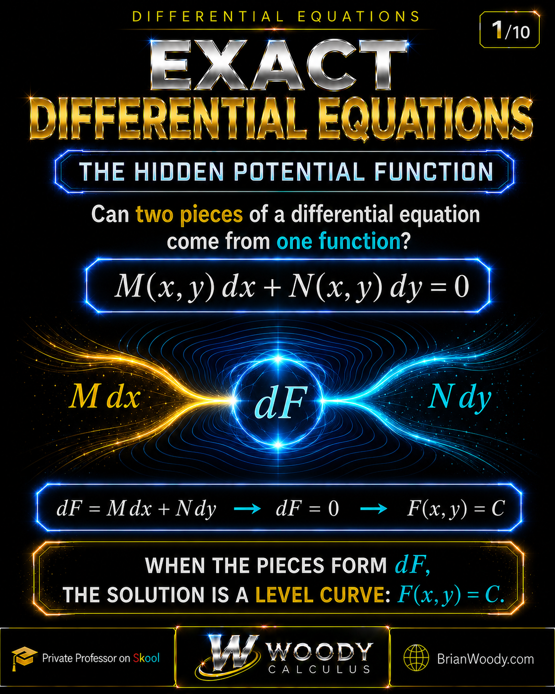
Learn how to recognize and solve exact differential equations using the exactness test M_y = N_x, recover a potential function F(x,y), apply initial conditions, verify implicit solutions, and use special integrating factors when an equation is not exact. This rigorous visual lesson also explains domain restrictions, conservative vector fields, line integrals, and the punctured-domain caveat.
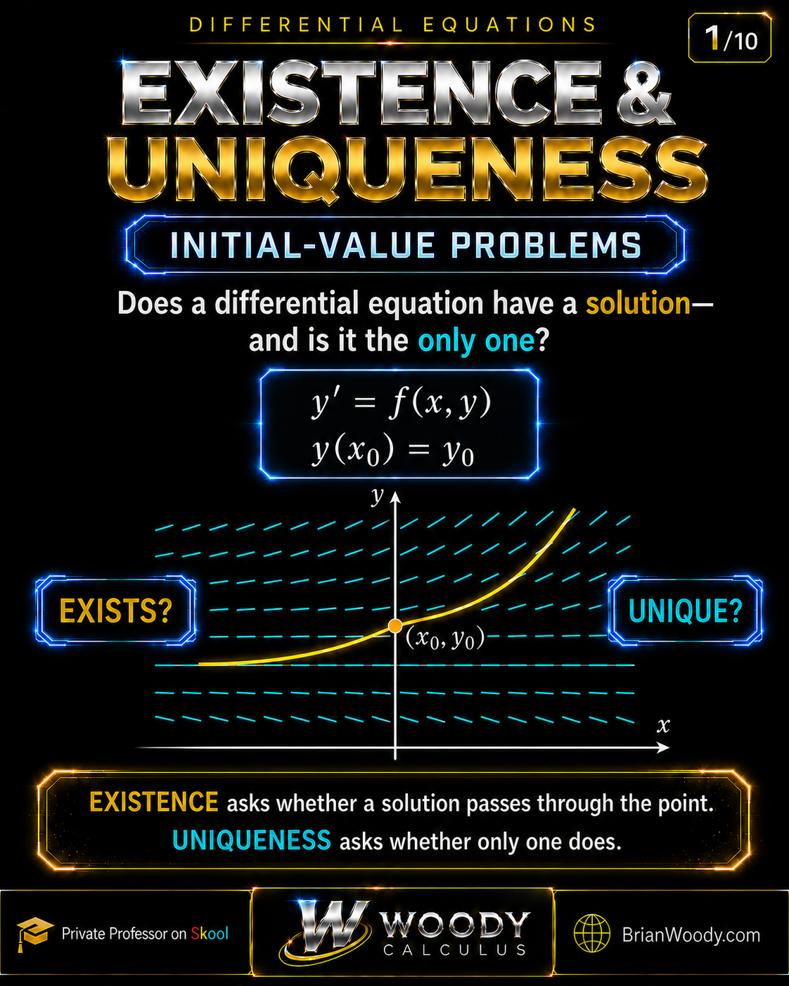
Does an initial-value problem have a solution, and is that solution the only one? This complete Woody Calculus lesson explains the existence and uniqueness theorem, the rectangle test, worked examples, nonunique solutions, finite-time blow-up, maximal intervals, the nonintersection principle, and higher-order linear ODEs.
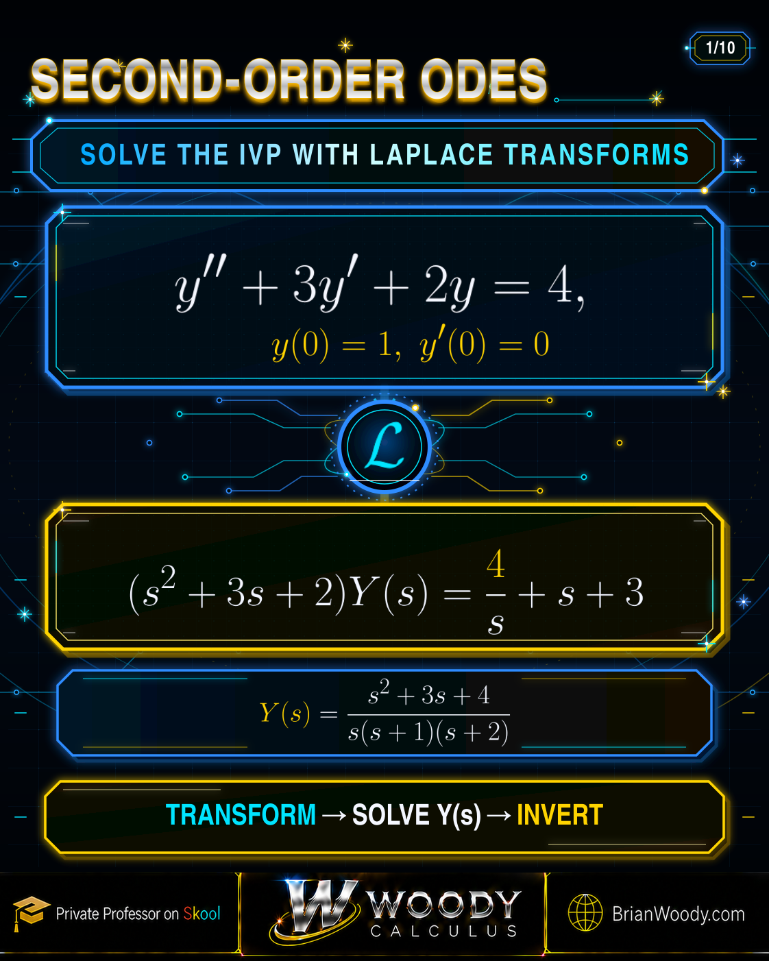
Laplace transforms turn second-order initial-value problems into algebra while carrying the initial conditions with them. Learn the complete seven-step method, partial fractions, delayed unit-step inputs, Dirac delta impulses, transfer functions, impulse response, convolution, stability, and verification through exact worked examples.
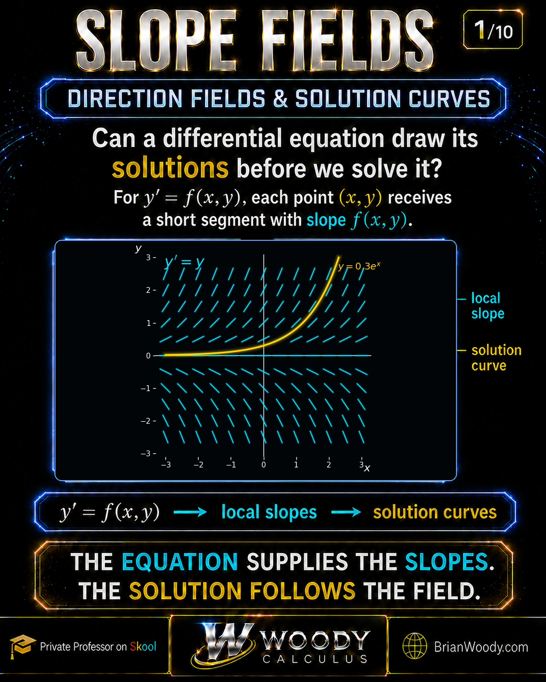
Slope fields make differential equations visible. Learn how to construct and read direction fields, use isoclines, sketch IVP solution curves, distinguish zero-slope curves from equilibria, understand uniqueness, analyze logistic stability, and apply Euler’s method through exact worked examples.
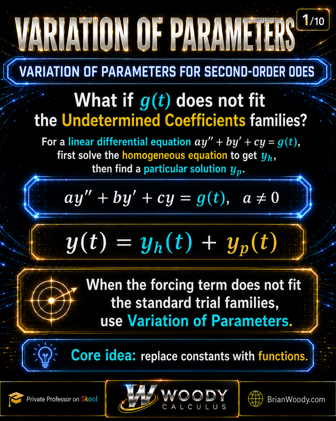
Differential Equations • Second-Order Linear ODEs • Visual Lesson Level: Undergraduate Differential Equations | Core skill: Find a particular solution…
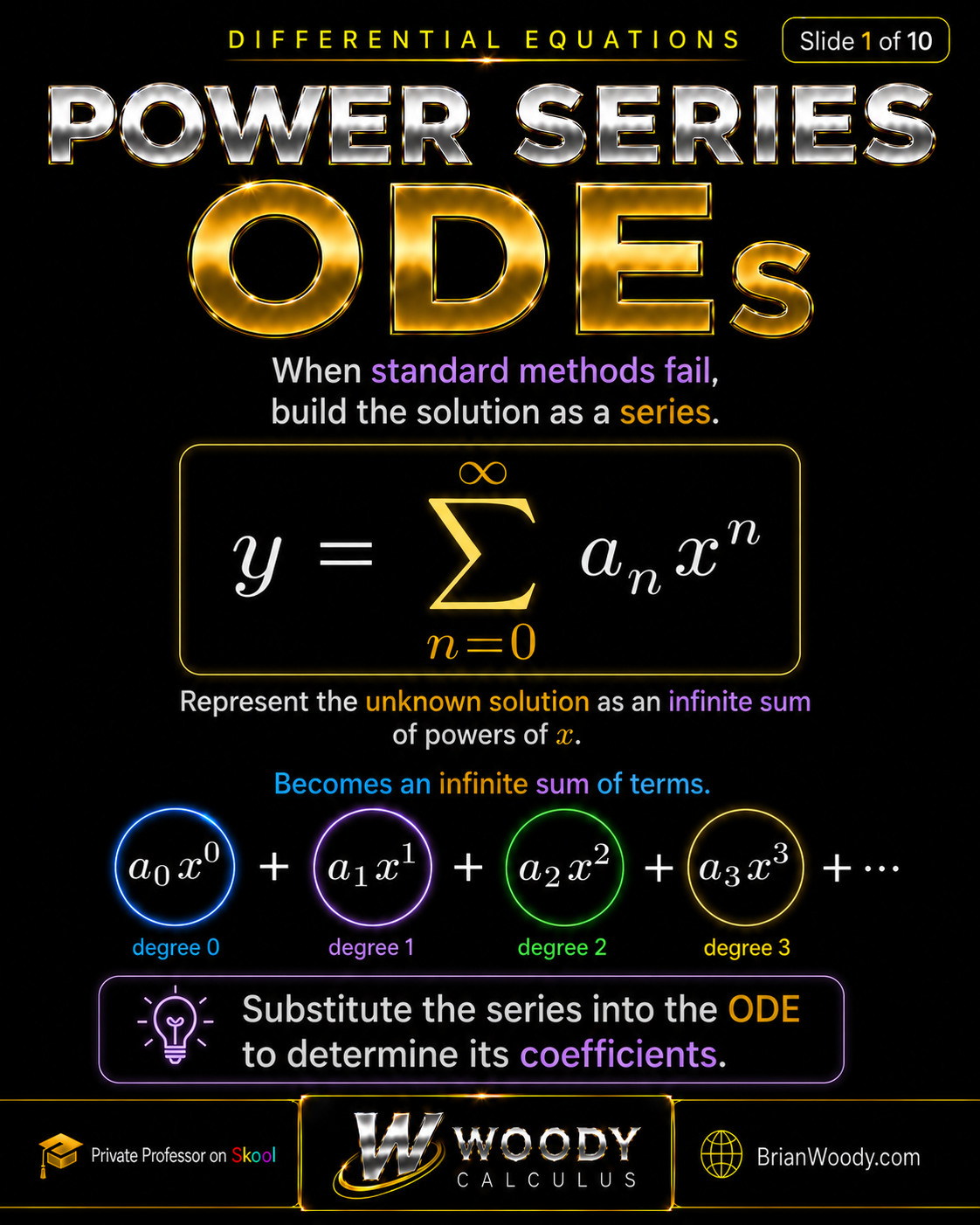
Learn how to solve differential equations with power series through a complete Airy equation example. This Woody Calculus lesson explains ordinary points, term-by-term differentiation, reindexing, recurrence relations, coefficient chains, initial conditions, and independent verification.
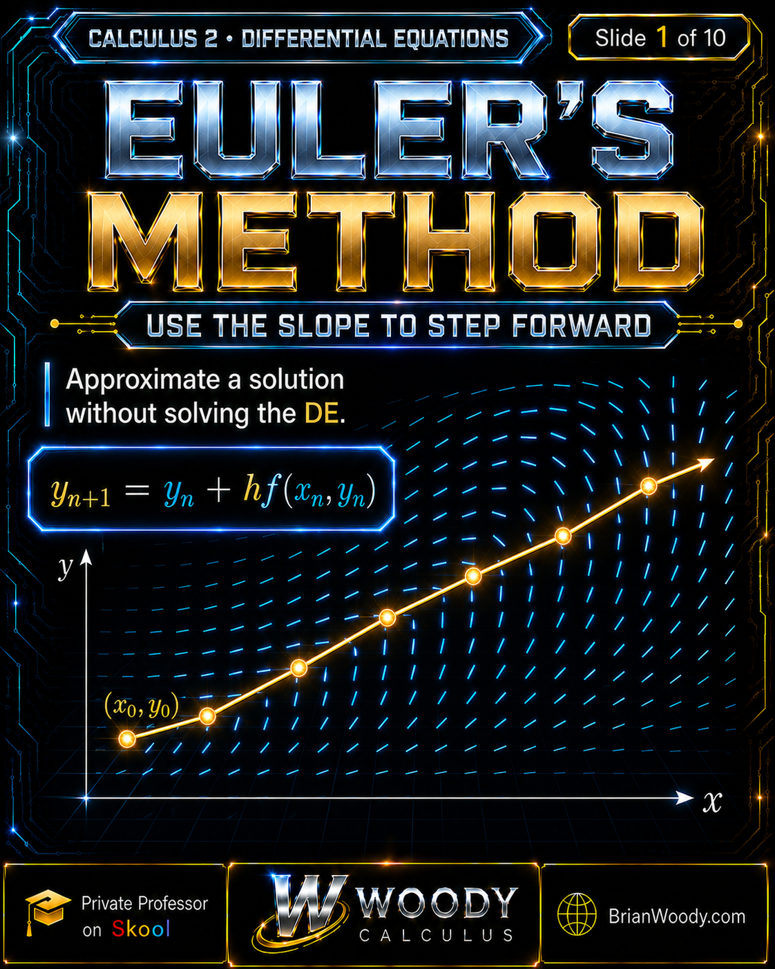
Euler’s method approximates the solution of an initial-value problem by repeatedly using the differential equation’s slope. Learn the update formula, complete a worked example, compare step sizes, and verify the approximation against an exact solution.
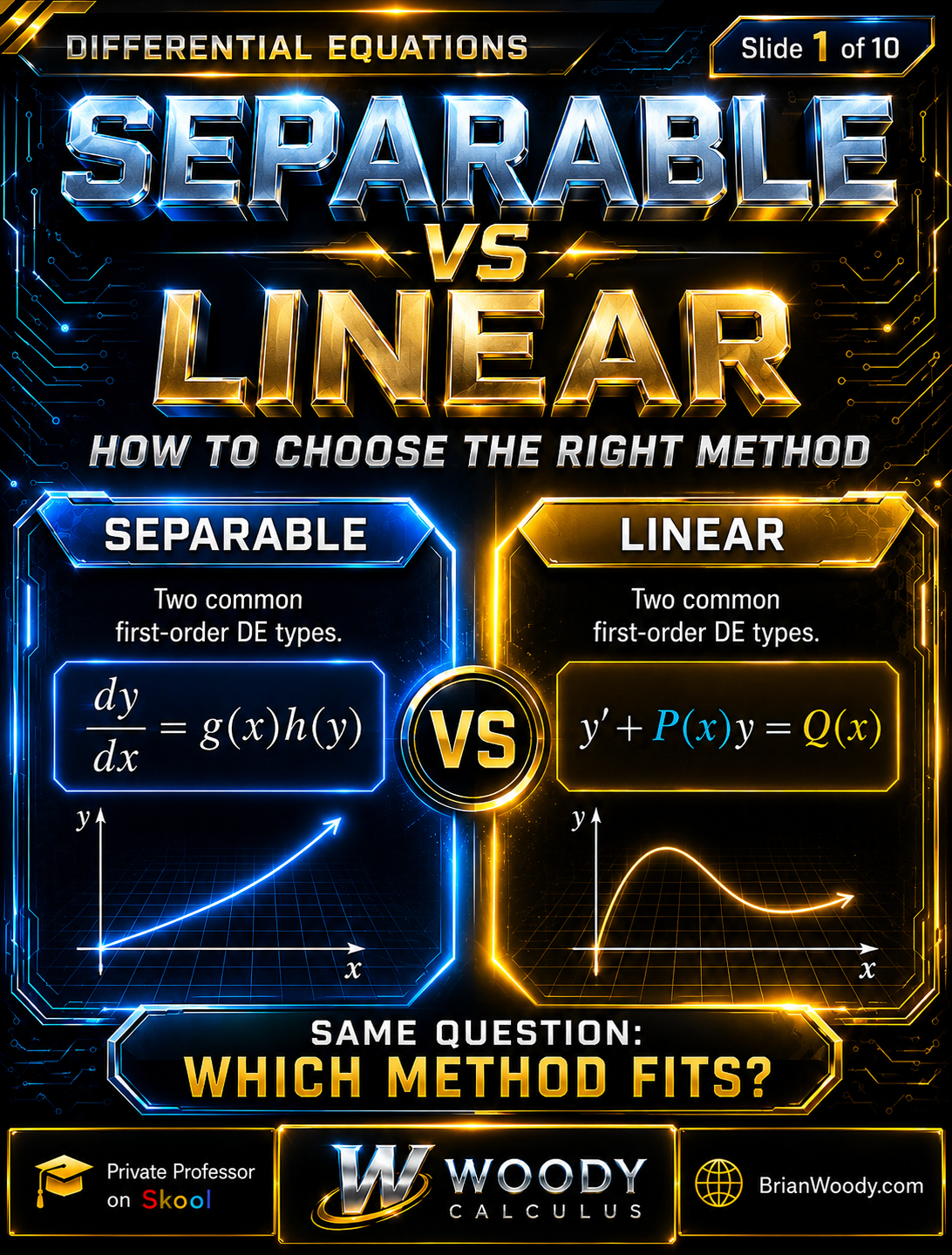
How do you decide whether to use separation of variables or an integrating factor? This Woody Calculus lesson explains how to classify separable and first-order linear differential equations, solve each type step by step, handle equations that fit both methods, and verify the final solution.
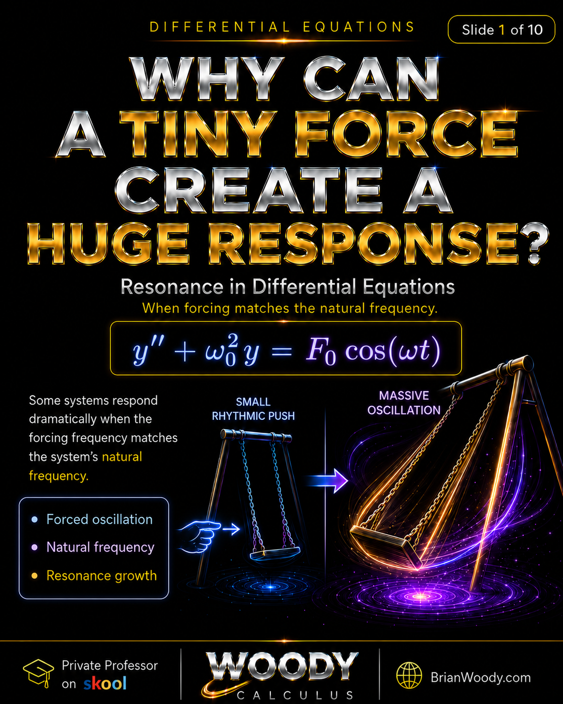
Resonance happens when a forcing frequency matches a system’s natural frequency. This Woody Calculus Differential Equations lesson explains forced oscillations, natural frequency, undamped resonance growth, damping, peak response, and real-world applications.