Resonance is one of the most powerful ideas in Differential Equations. It explains why a tiny repeated force can create a huge response when the timing is exactly right.
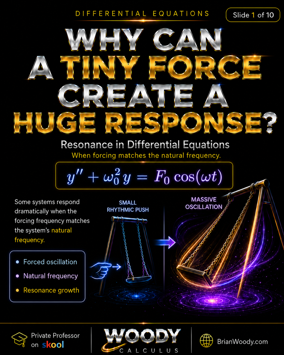
A child on a swing is the classic example. One small push does not do much. But if every push arrives at the right moment, the motion grows larger and larger. That is resonance.
In Differential Equations, resonance occurs when the forcing frequency matches the system’s natural frequency. In the undamped case, that perfect match can create amplitude growth over time.
Resonance is not about force size first. Resonance is about timing.
This Woody Calculus lesson teaches resonance through the forced oscillator model, natural frequency, nonresonant bounded motion, exact resonance growth, and the role of damping in real systems. Mathematically, this topic belongs to ordinary differential equations, second-order linear ODEs, and the study of the driven harmonic oscillator.
Students studying resonance should also connect this topic to Laplace transforms, eigenvalues and eigenvectors, Fourier series, and the broader study of transient response, steady-state response, and linear systems in Differential Equations.
Estimated read time: 10–13 minutes.
Last updated: July 9, 2026.
Quick Summary: Resonance in Differential Equations
- Resonance happens when the forcing frequency matches the natural frequency.
- The standard forced oscillator model is \(m y^{\prime\prime}+c y^{\prime}+ky=F_0\cos(\omega t)\).
- Without damping and forcing, the system oscillates naturally at \(\omega_0=\sqrt{k/m}\).
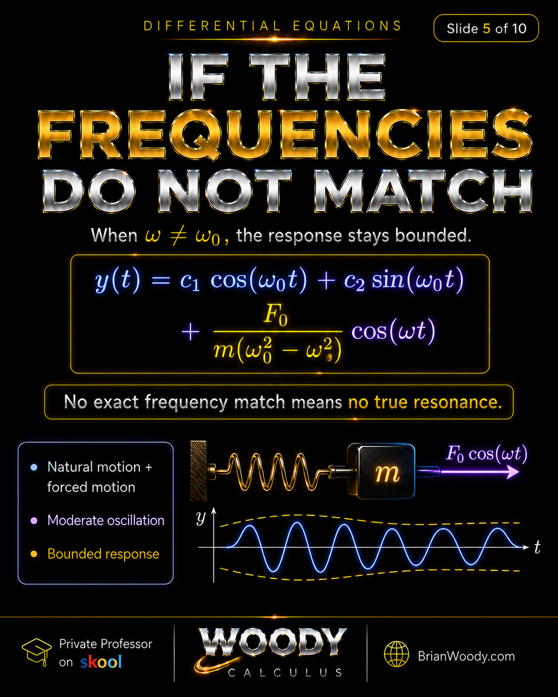
- When \(\omega\ne \omega_0\), the undamped forced response stays bounded.
- When \(\omega=\omega_0\), exact resonance occurs.
- At exact undamped resonance, the solution contains a factor of \(t\), so the amplitude grows over time.
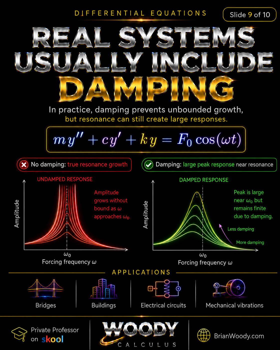
- Real systems usually include damping, which prevents unbounded growth but still creates large peak responses near resonance.
- Resonance appears in bridges, buildings, circuits, mechanical vibrations, musical instruments, and engineering systems.
Resonance Key Facts
- Natural frequency is the system’s built-in rhythm.
- Forcing frequency is the frequency of the external input.
- Resonance occurs when the forcing frequency matches the natural frequency.
- For an undamped spring-mass system, \(\omega_0=\sqrt{k/m}\).
- In the undamped nonresonant case, the particular solution has denominator \(\omega_0^2-\omega^2\).
- At resonance, the usual particular solution fails because the forcing matches the homogeneous motion.
- In practical damped systems, resonance produces a large but finite peak response near the natural frequency.
- This topic is central to Differential Equations, Laplace transforms, vibration analysis, and engineering mathematics.
What Is Resonance?
Resonance is a phenomenon in which a system responds strongly to an external force because the external force is applied at the system’s natural frequency.
In Differential Equations, resonance usually appears in second-order linear equations that model oscillation. The basic idea is:
\text{forcing frequency}=\text{natural frequency}.
\]
When the timing matches perfectly, energy is added efficiently cycle after cycle. In an ideal undamped model, this creates amplitude growth without bound.
In normalized form, a basic undamped forced oscillator can be written as:
y^{\prime\prime}+\omega_0^2 y=A\cos(\omega t),
\]
where \(\omega_0\) is the natural frequency, \(\omega\) is the forcing frequency, and \(A=\frac{F_0}{m}\) after dividing the physical equation by the mass.
The dramatic case occurs when:
\omega=\omega_0.
\]
The Forced Oscillation Model
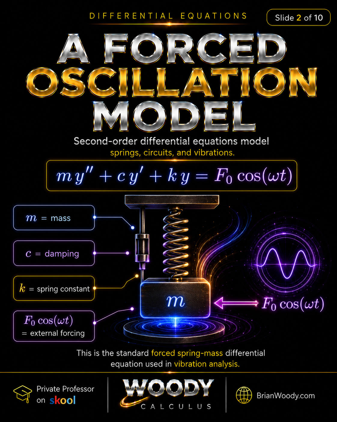
The standard physical model for a forced spring-mass system is:
m y^{\prime\prime}+c y^{\prime}+ky=F_0\cos(\omega t).
\]
Each term has a physical meaning:
- \(m\) is the mass.
- \(c\) is the damping coefficient.
- \(k\) is the spring constant.
- \(F_0\cos(\omega t)\) is the external periodic force.
This same structure appears in mechanical vibrations, electrical circuits, building motion, bridge oscillations, and engineering systems.
Every System Has Its Own Rhythm
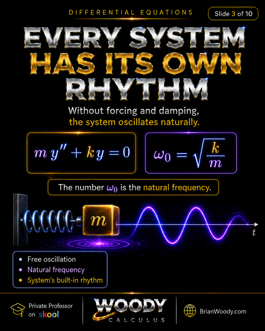
Before forcing is added, consider the undamped free oscillator:
m y^{\prime\prime}+ky=0.
\]
Divide by \(m\):
y^{\prime\prime}+\frac{k}{m}y=0.
\]
The natural frequency is:
\omega_0=\sqrt{\frac{k}{m}}.
\]
So the free oscillator satisfies:
y^{\prime\prime}+\omega_0^2 y=0.
\]
Its general solution is:
y(t)=c_1\cos(\omega_0 t)+c_2\sin(\omega_0 t).
\]
This is the system’s built-in rhythm. If nothing drives the system from outside, it naturally oscillates at frequency \(\omega_0\).
Now Add an Outside Force
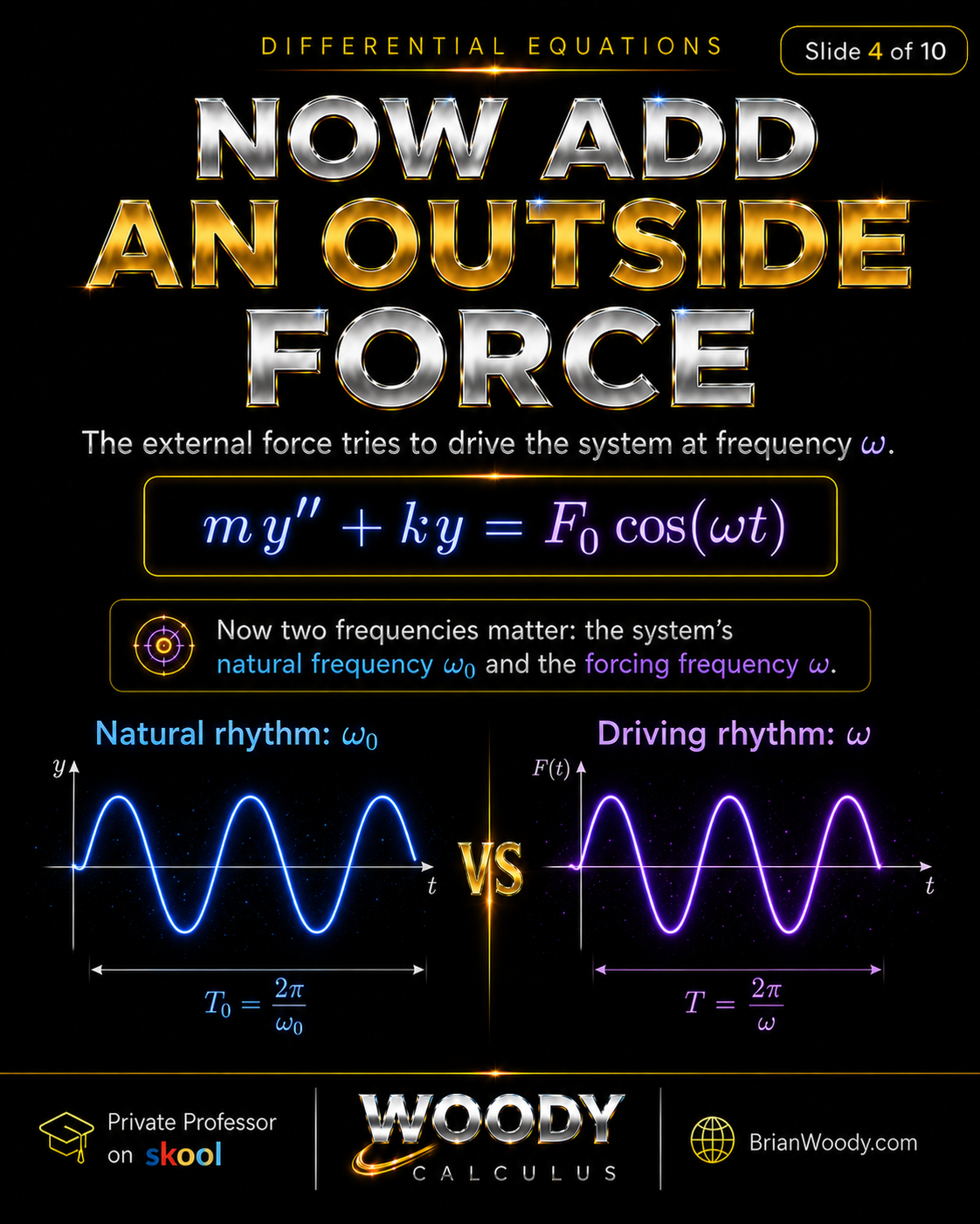
Now add an external periodic force:
m y^{\prime\prime}+ky=F_0\cos(\omega t).
\]
There are now two frequencies:
- \(\omega_0\), the natural frequency of the system,
- \(\omega\), the forcing frequency of the external input.
The entire resonance story depends on how these two frequencies compare.
If \(\omega\ne\omega_0\), the response stays bounded in the ideal undamped model. If \(\omega=\omega_0\), the external force is perfectly synchronized with the natural motion, and true resonance occurs.
If the Frequencies Do Not Match
For the undamped forced equation:
m y^{\prime\prime}+ky=F_0\cos(\omega t),
\]
write:
\omega_0^2=\frac{k}{m}.
\]
If \(\omega\ne\omega_0\), a particular solution has the form:
y_p(t)=\frac{F_0}{m(\omega_0^2-\omega^2)}\cos(\omega t).
\]
Therefore the full solution is:
y(t)=c_1\cos(\omega_0 t)+c_2\sin(\omega_0 t)
+
\frac{F_0}{m(\omega_0^2-\omega^2)}\cos(\omega t).
\]
This response is bounded when \(\omega\ne\omega_0\). The denominator \(\omega_0^2-\omega^2\) explains why the amplitude gets large when \(\omega\) is close to \(\omega_0\).
No exact frequency match means no true undamped resonance.
Resonance Equals Perfect Frequency Match
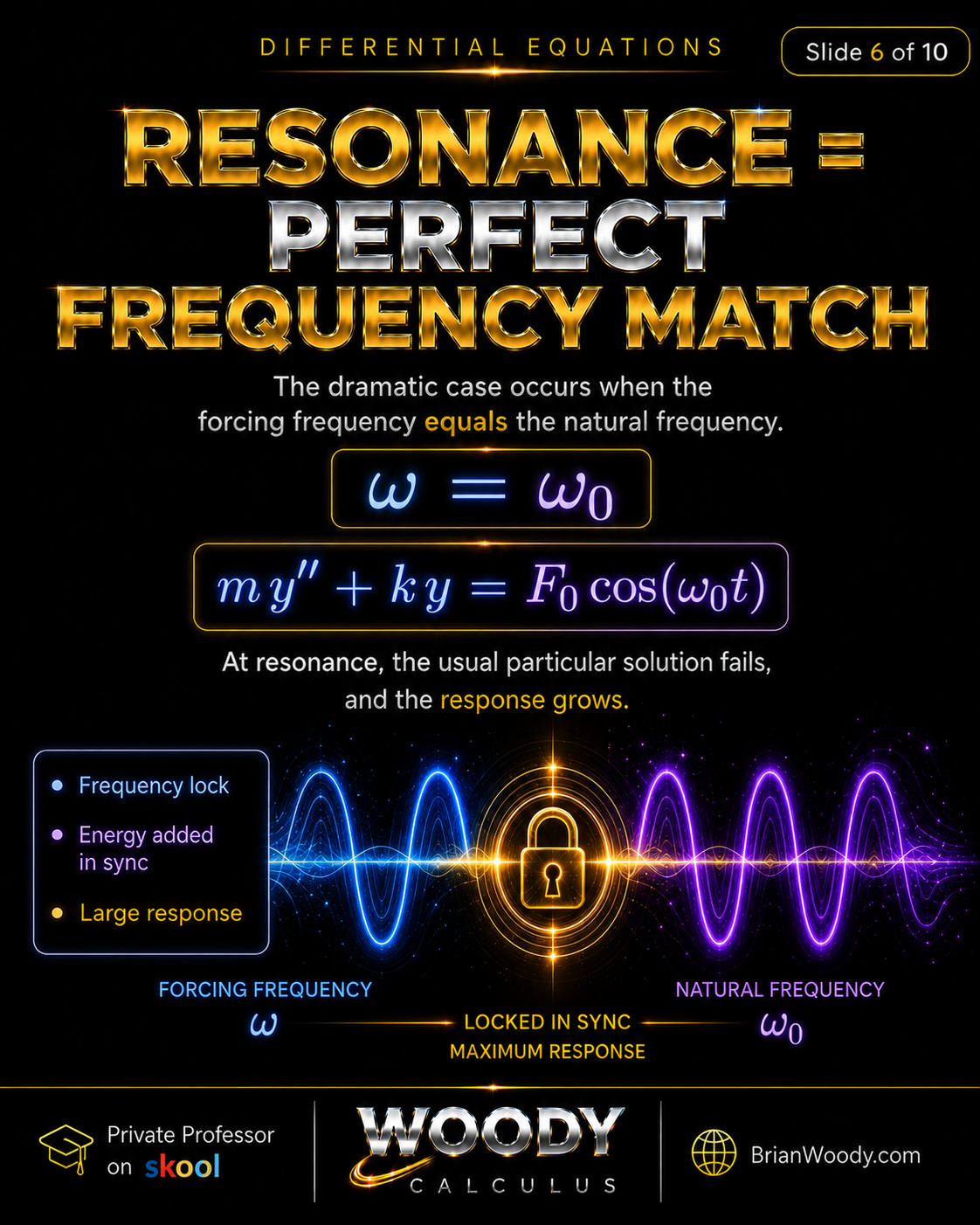
The dramatic case occurs when:
\omega=\omega_0.
\]
Then the forced equation becomes:
m y^{\prime\prime}+ky=F_0\cos(\omega_0 t).
\]
The usual particular solution form \(A\cos(\omega t)\) fails because \(\cos(\omega_0 t)\) is already part of the homogeneous solution.
In Differential Equations language, the forcing term duplicates the natural mode. That duplication creates resonance.
At resonance, the external force pushes the system at exactly its own natural rhythm.
What the Solution Looks Like at Resonance
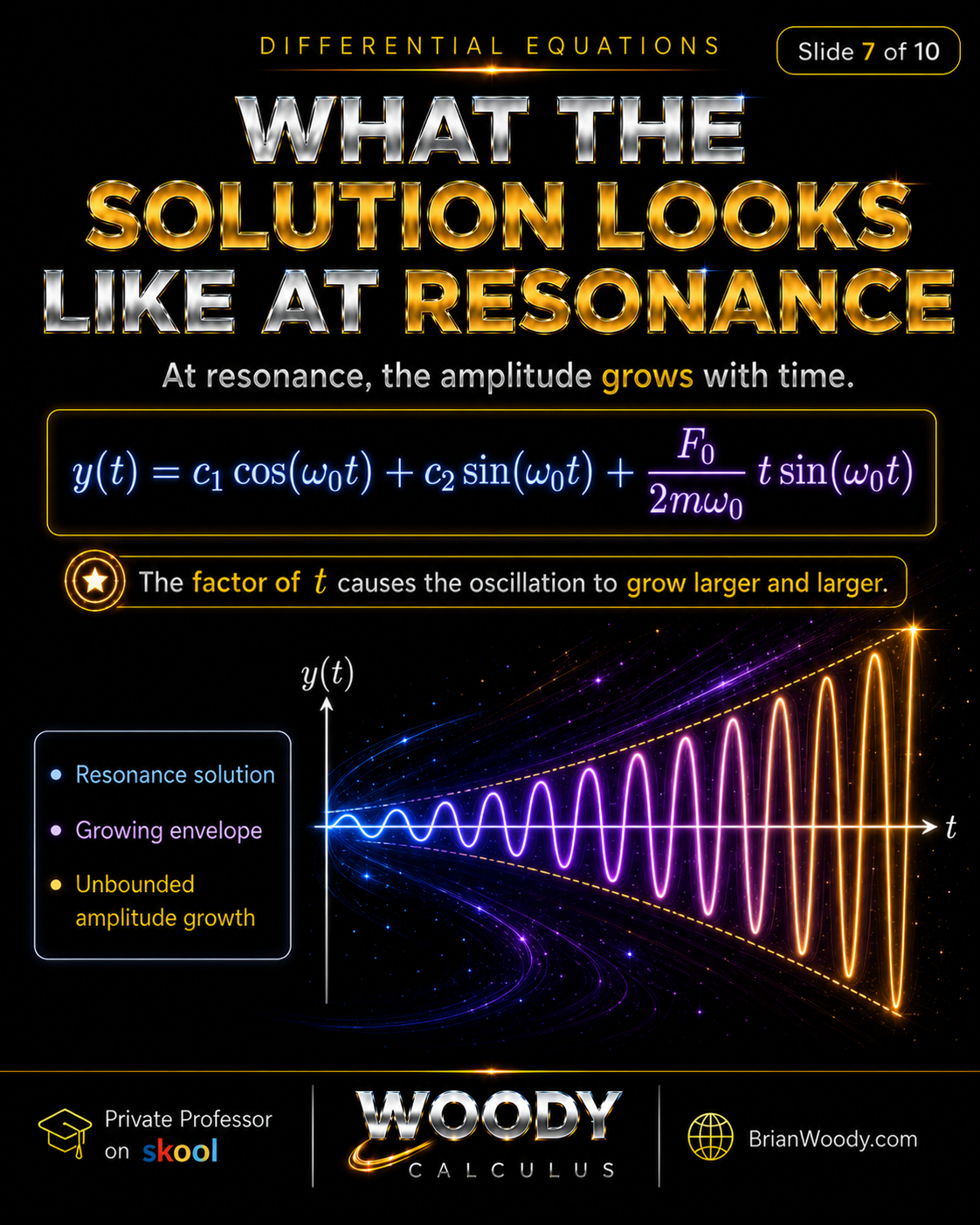
At exact undamped resonance, the solution becomes:
y(t)=c_1\cos(\omega_0 t)+c_2\sin(\omega_0 t)
+
\frac{F_0}{2m\omega_0}t\sin(\omega_0 t).
\]
The important part is the factor of \(t\):
\frac{F_0}{2m\omega_0}t\sin(\omega_0 t).
\]
The sine function oscillates, but the coefficient grows linearly with time. That means the amplitude grows larger and larger in the ideal undamped model.
This is why resonance can be so dramatic: the force does not need to be huge. It only needs to be applied at the right frequency.
Timing Beats Strength
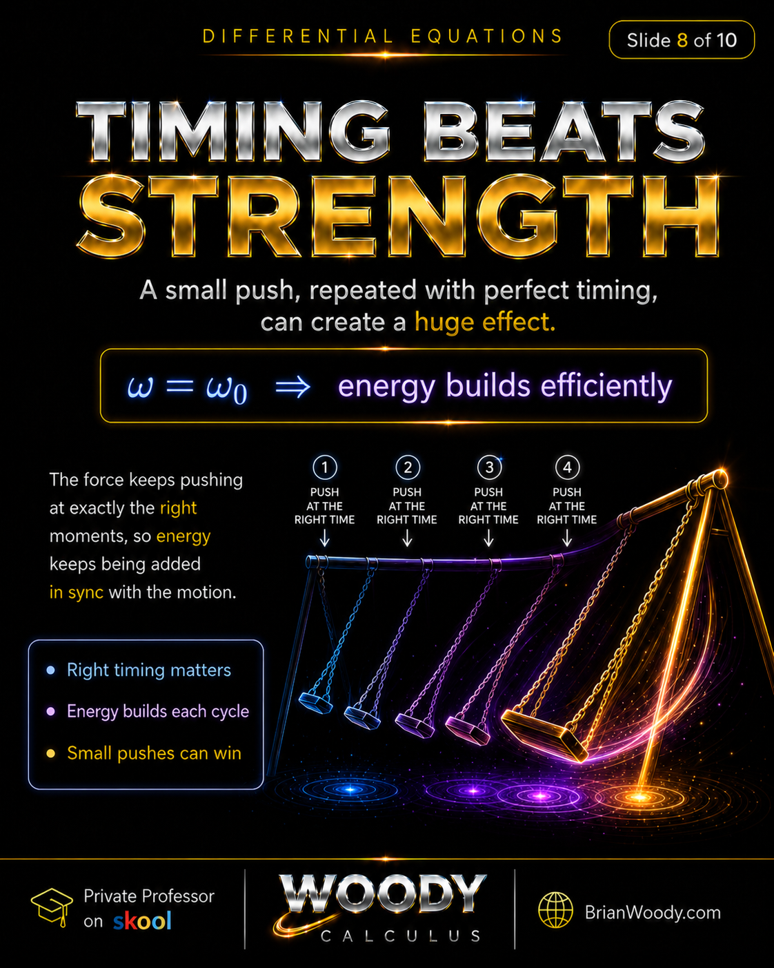
Resonance is the mathematics of timing.
A small push on a swing can create a large effect when it is repeated at exactly the right time. Each push adds energy in sync with the motion.
\omega=\omega_0
\quad\Longrightarrow\quad
\text{energy builds efficiently}.
\]
This is why a small periodic force can be more powerful than a large poorly timed force.
In resonance, timing beats strength.
Real Systems Usually Include Damping
Real systems usually include damping:
m y^{\prime\prime}+c y^{\prime}+ky=F_0\cos(\omega t).
\]
When \(c>0\), damping removes energy from the system. This prevents unbounded resonance growth.
However, damping does not make resonance disappear. It changes the picture:
- With no damping, exact resonance can produce unbounded amplitude growth.
- With damping, the response remains finite.
- With light damping, the response can still have a large peak near the natural frequency.
For a damped forced oscillator, the steady-state amplitude has the form:
A(\omega)=
\frac{F_0}
{\sqrt{(k-m\omega^2)^2+(c\omega)^2}}.
\]
This formula shows why damping matters. The term \(c\omega\) prevents the denominator from becoming zero, so the amplitude remains finite.
With light damping, specifically when \(c^2<2mk\), the peak response occurs at:
\omega_{\text{peak}}
=
\sqrt{\omega_0^2-\frac{c^2}{2m^2}}.
\]
This peak frequency is slightly below \(\omega_0\), and it moves lower as damping increases. That is why the corrected damped-resonance picture shows a large finite peak near the natural frequency, not an infinite spike exactly at \(\omega_0\).
That is why real systems such as bridges, buildings, engines, circuits, and mechanical devices are designed with damping in mind.
Worked Example: Resonance in an Undamped Oscillator
Solve the forced oscillator:
y^{\prime\prime}+9y=4\cos(3t).
\]
Here:
\omega_0^2=9,
\qquad
\omega_0=3.
\]
The forcing term is:
4\cos(3t),
\]
so the forcing frequency is:
\omega=3.
\]
Thus:
\omega=\omega_0.
\]
This is exact resonance.
The homogeneous solution is:
y_h(t)=c_1\cos(3t)+c_2\sin(3t).
\]
For:
y^{\prime\prime}+\omega_0^2y=A\cos(\omega_0 t),
\]
the resonant particular solution is:
y_p(t)=\frac{A}{2\omega_0}t\sin(\omega_0 t).
\]
Here \(A=4\) and \(\omega_0=3\), so:
y_p(t)=\frac{4}{2(3)}t\sin(3t)
=
\frac{2}{3}t\sin(3t).
\]
Therefore:
\boxed{
y(t)=c_1\cos(3t)+c_2\sin(3t)+\frac23 t\sin(3t).
}
\]
Plain-language formula: The resonant solution to \(y^{\prime\prime}+9y=4\cos(3t)\) is \(c_1\cos(3t)+c_2\sin(3t)+\frac23 t\sin(3t)\), and the factor of \(t\) causes amplitude growth.
Common Mistakes
Mistake 1: Confusing natural frequency and forcing frequency
The natural frequency \(\omega_0\) comes from the system itself. The forcing frequency \(\omega\) comes from the external input.
Mistake 2: Forgetting to compare frequencies
Before solving a forced oscillator, always compare:
\omega
\qquad
\text{and}
\qquad
\omega_0.
\]
If they match, resonance is possible.
Mistake 3: Using the nonresonant formula at resonance
The nonresonant particular solution contains:
\frac{1}{\omega_0^2-\omega^2}.
\]
At resonance, \(\omega=\omega_0\), so this denominator becomes zero. A different particular solution is needed.
Mistake 4: Forgetting the factor of \(t\)
At exact undamped resonance, the solution contains:
t\sin(\omega_0 t).
\]
That factor of \(t\) is what produces amplitude growth.
Mistake 5: Thinking all real resonance is unbounded
Real systems usually have damping. Damping prevents unbounded growth, but it can still allow a large finite peak response near the natural frequency.
Resonance Cheat Sheet
| Case | Equation | Behavior | Key Idea |
|---|---|---|---|
| Free undamped oscillator | \(m y^{\prime\prime}+ky=0\) | Natural oscillation | \(\omega_0=\sqrt{k/m}\) |
| Forced nonresonant oscillator | \(m y^{\prime\prime}+ky=F_0\cos(\omega t)\), \(\omega\ne\omega_0\) | Bounded response | No exact frequency match |
| Forced resonant oscillator | \(m y^{\prime\prime}+ky=F_0\cos(\omega_0 t)\) | Amplitude grows | \(t\sin(\omega_0 t)\) appears |
| Damped forced oscillator | \(m y^{\prime\prime}+c y^{\prime}+ky=F_0\cos(\omega t)\) | Finite peak response | Damping prevents unbounded growth |
Resonance FAQ
What is resonance in Differential Equations?
Resonance is the large response that occurs when the forcing frequency of an external input matches the natural frequency of a system.
What is natural frequency?
Natural frequency is the frequency at which a system oscillates on its own without external forcing. For an undamped spring-mass system, \(\omega_0=\sqrt{k/m}\).
What is forcing frequency?
Forcing frequency is the frequency of an external periodic input, such as \(F_0\cos(\omega t)\). The forcing frequency is \(\omega\).
When does resonance occur?
In the ideal undamped model, resonance occurs when the forcing frequency equals the natural frequency, so \(\omega=\omega_0\).
Why does amplitude grow at resonance?
At exact undamped resonance, the particular solution contains a factor of \(t\), such as \(t\sin(\omega_0 t)\). That factor causes the oscillation amplitude to grow over time.
What happens when the frequencies do not match?
When \(\omega\ne\omega_0\), the undamped forced response stays bounded and the system does not experience true resonance.
How does damping affect resonance?
Damping prevents unbounded resonance growth. A damped system can still have a large finite response near the natural frequency, but the amplitude remains bounded.
Where does resonance appear in real life?
Resonance appears in bridges, buildings, electrical circuits, mechanical vibrations, musical instruments, engines, and many engineering systems.
Master Differential Equations with Woody Calculus
Resonance is one of the clearest examples of why Differential Equations matters. A simple equation can explain a dramatic physical effect.
The Woody Calculus method is:
- Identify the model.
- Find the natural frequency.
- Identify the forcing frequency.
- Compare \(\omega\) and \(\omega_0\).
- Use the nonresonant formula when \(\omega\ne\omega_0\).
- Use the resonant \(t\sin(\omega_0 t)\) structure when \(\omega=\omega_0\).
- Account for damping in real systems.
The Woody Calculus method requires strict discipline. To master resonance, you must rely on deliberate formula memorization, rewrite perfect solutions from scratch, and vocalize each step out loud until the frequency comparison becomes automatic. Memorization is not the enemy of understanding; it is required.
For students who want structured Differential Equations help, join the Woody Calculus Mastery Lab. The Mastery Lab helps students build skill through repetition, step-by-step lessons, written solutions, exam-focused systems, and direct support.
You can also visit Woody Calculus on Skool for the learning community.
Related Woody Calculus Mathematical Essays
Explore more Woody Calculus lessons connecting Differential Equations, Laplace Transforms, Linear Algebra, Fourier Series, Calculus 2, Calculus 3, and advanced mathematics.
- How to Learn Calculus and Advanced Mathematics: A Peak Performance Study Guide
- Laplace Transforms Explained: Differential Equations Become Algebra
- Eigenvalues and Eigenvectors Explained
- The Determinant Explained
- Fourier Series Explained: Harmonics, Sound, Heat, and Quantum Mechanics
- Differential Equations and Chaos Theory: The Lorenz System
- Integration by Parts Explained: The Woody Calculus 3-Type System
- Trig Substitution Explained: The Woody Calculus 3-Type System
- View All Woody Calculus Blog Posts
Private Instruction
Brian M. Woody works privately with a limited number of serious students who need one-on-one help in Differential Equations, Calculus II, Calculus III, Linear Algebra, and advanced mathematics.
Private instruction is reserved for serious students, requires weekly sessions, requires enrollment in the Woody Calculus Mastery Lab first, and approval is not guaranteed.
Students interested in private instruction can learn more here: Private Math Tutor and Advanced Mathematics Instruction.
Related University Math Help Pages
Woody Calculus supports students at major universities with structured help in Differential Equations, Calculus 2, Calculus 3, Linear Algebra, and advanced mathematics. For the full list of supported schools, visit the University Calculus Tutor Hub.
- University Calculus Tutor Hub
- Purdue University Calculus Tutor
- University of Florida Calculus Tutor
- Colorado State University Calculus Help
- UCF Calculus Tutor
- University of Nevada, Reno Calculus Tutor
- Auburn Calculus Tutor
- University of Alabama Calculus Tutor
- University of Wisconsin Calculus Tutor
- University of Michigan Calculus Tutor
- UCLA Calculus Tutor
- MIT Calculus Tutor
Trusted by Students Nationwide
The Woody Calculus Mastery Lab gives university students access to structured mathematics support, written solutions, video lessons, exam-focused training, and expert guidance from Brian M. Woody.
Students use Woody Calculus for Differential Equations, Calculus II, Calculus III, Linear Algebra, Abstract Algebra, and other advanced mathematics courses.