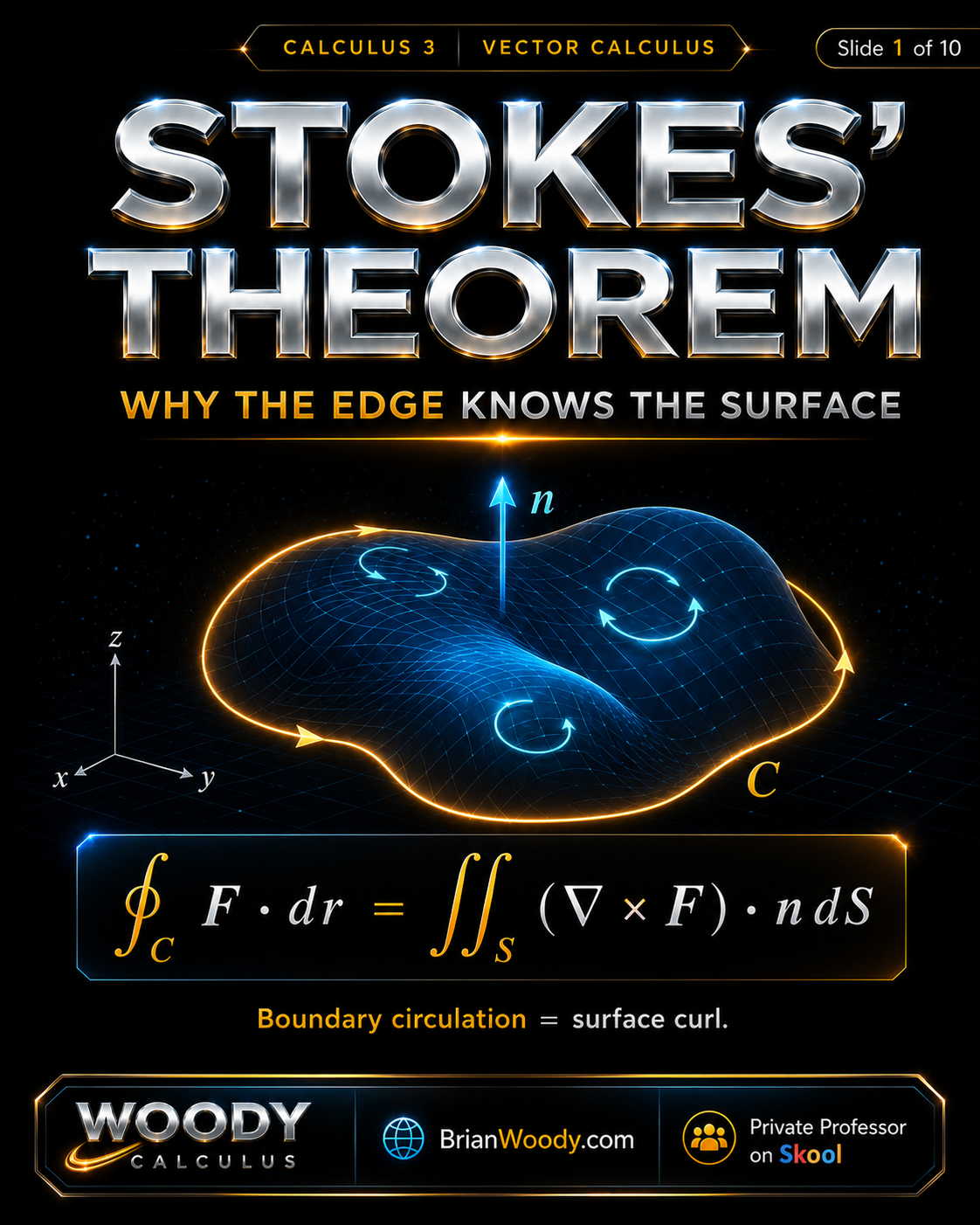
Stokes’ Theorem says that boundary circulation equals the total curl through a surface. In this Woody Calculus visual lesson, learn how Stokes’ Theorem connects line integrals, surface integrals, curl, orientation, the right-hand rule, Green’s Theorem, and vector calculus in Calculus 3.
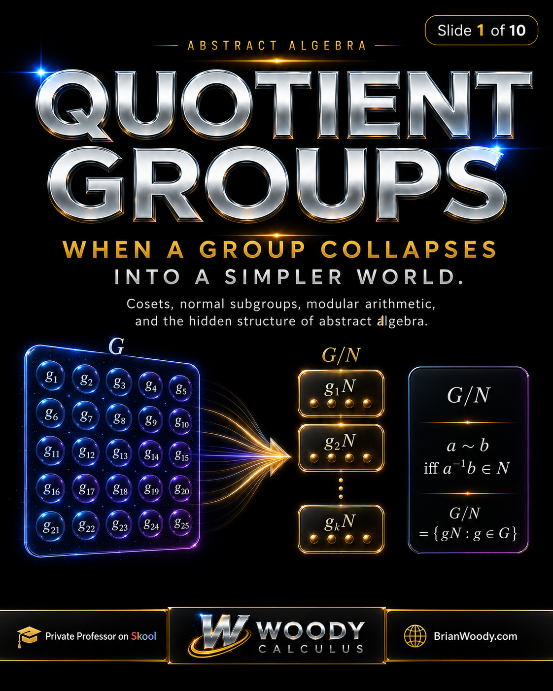
Quotient groups are how Abstract Algebra collapses a group into a simpler structure. In this Woody Calculus visual lesson, learn how cosets become the new elements, why normal subgroups are required, how modular arithmetic is a quotient group, and how kernels lead directly to the First Isomorphism Theorem.
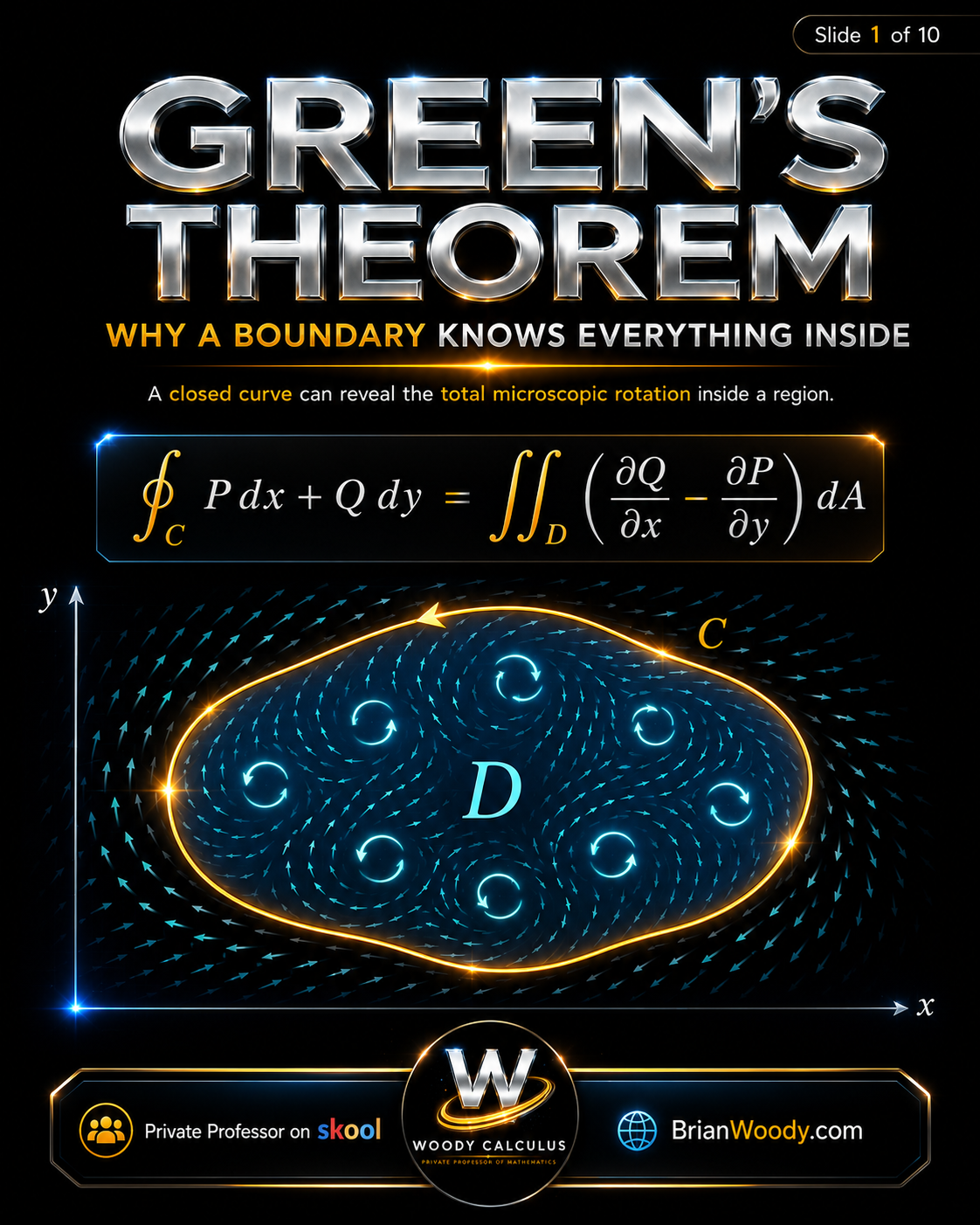
Green’s Theorem turns a boundary line integral into an interior double integral. In this Woody Calculus visual lesson, learn how Green’s Theorem connects circulation, curl, flux, area, line integrals, double integrals, Stokes’ Theorem, and the Divergence Theorem in Calculus 3.
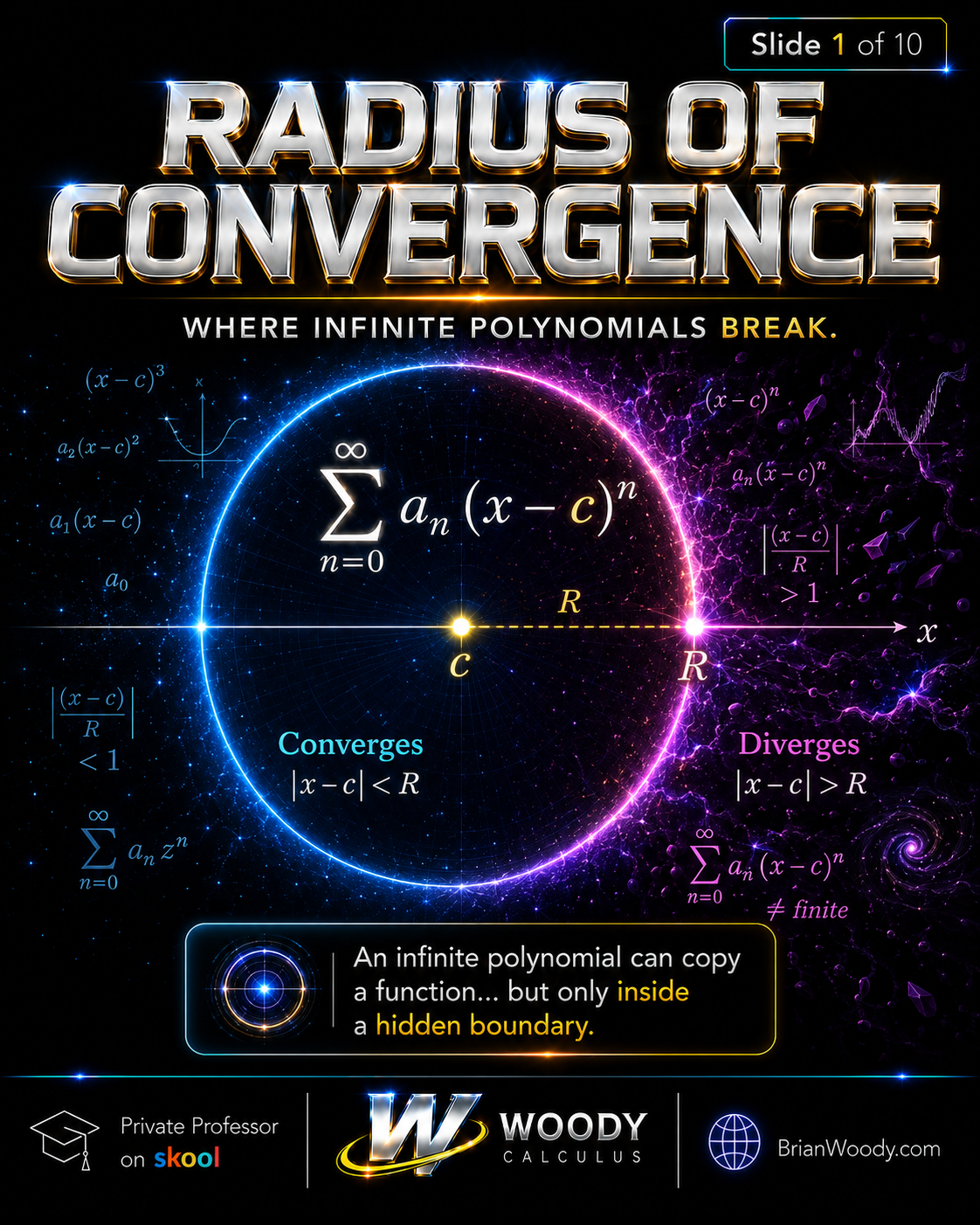
The radius of convergence is the hidden boundary where an infinite polynomial stops behaving like a function. In this Woody Calculus visual lesson, learn how power series are built around a center, how the Ratio Test finds R, why endpoints must be tested separately, and how to find the full interval of convergence.
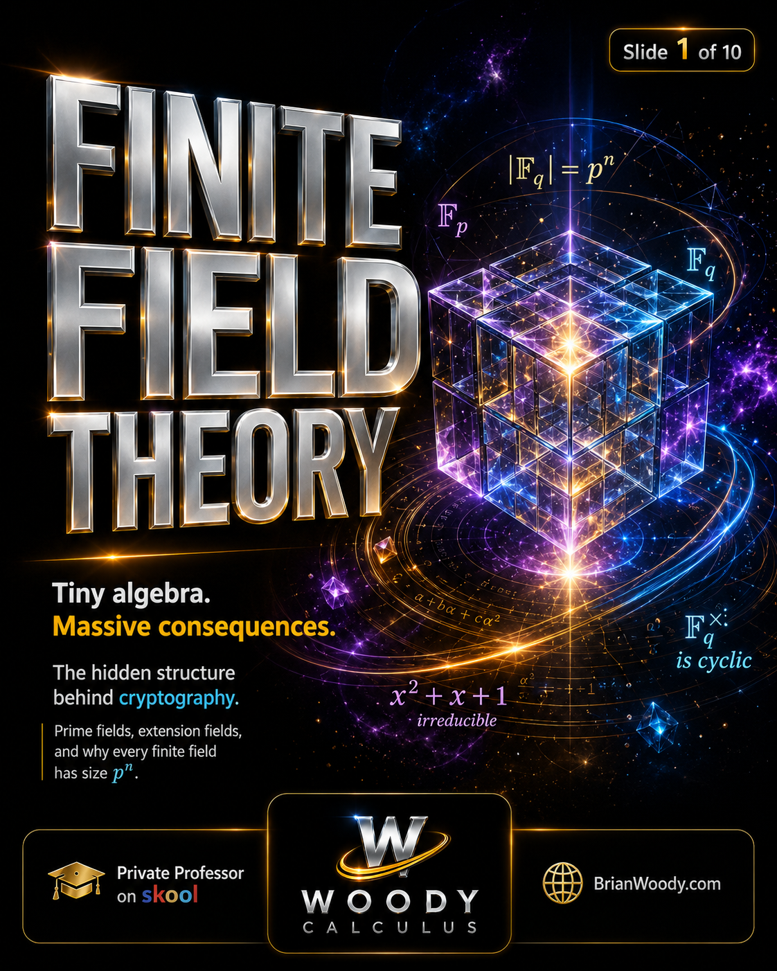
Finite field theory looks abstract until you realize it powers modern cryptography, error correction, QR codes, AES encryption, and elliptic curve cryptography. In this Woody Calculus visual lesson, learn what finite fields are, why prime fields matter, why every finite field has size q = p^n, how extension fields are built from irreducible polynomials, and why finite fields are the hidden algebra behind secure communication.
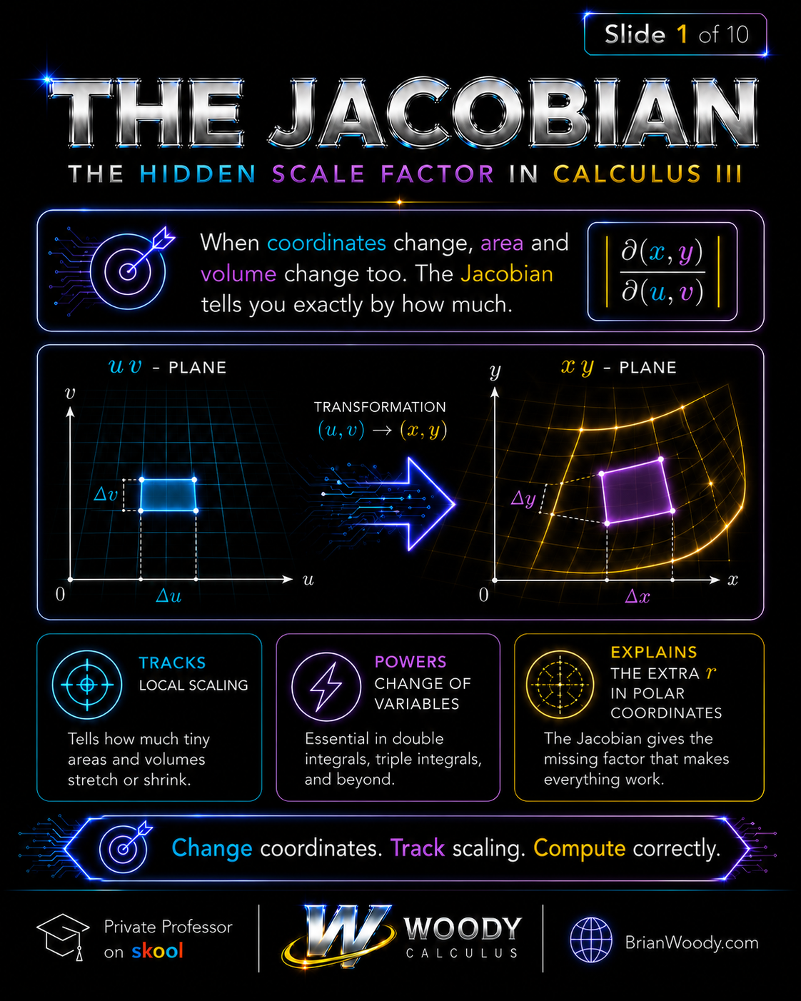
The Jacobian is the hidden scale factor behind every coordinate change in Calculus III. In this Woody Calculus visual lesson, learn how Jacobians explain area and volume scaling, change of variables, polar coordinates, cylindrical coordinates, spherical coordinates, double integrals, triple integrals, and why the mysterious extra factors r and ρ²sinφ appear.
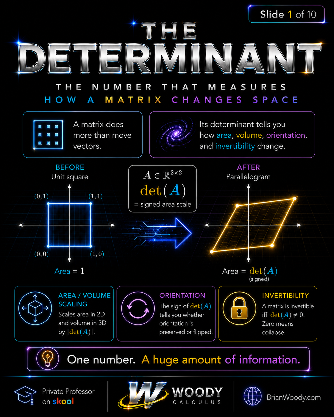
The determinant is the number that measures how a matrix changes space. In this Woody Calculus visual lesson, learn how determinants explain area and volume scaling, orientation, invertibility, matrix collapse, eigenvalues, Wronskians, and why det(A) connects Linear Algebra to Differential Equations.
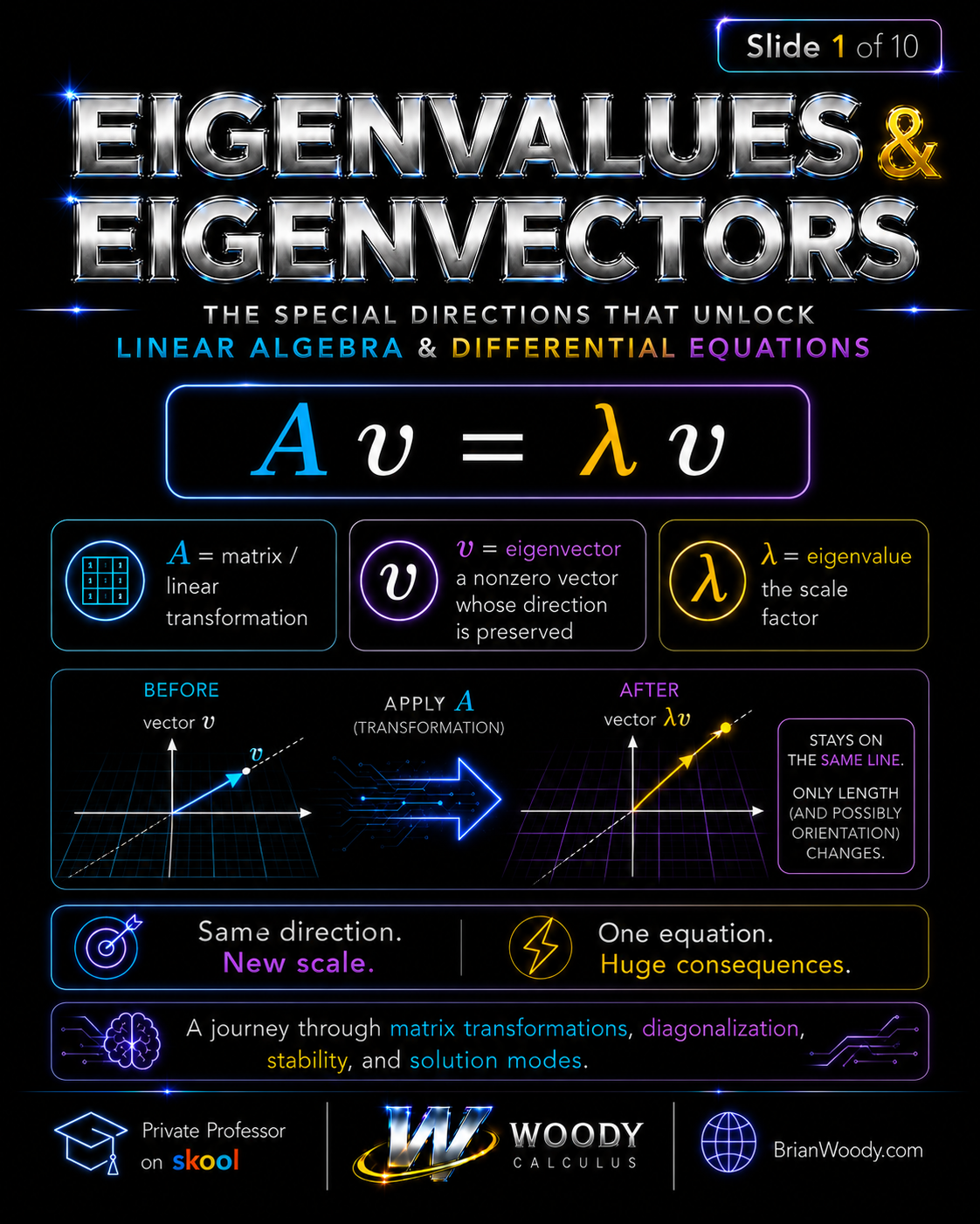
Eigenvalues and eigenvectors reveal the special directions that unlock Linear Algebra and Differential Equations. In this Woody Calculus visual lesson, learn how Av = λv explains matrix transformations, scaling, diagonalization, matrix powers, solution modes, stability, phase portraits, and why eigenvalues predict long-term behavior in systems before you even solve them.
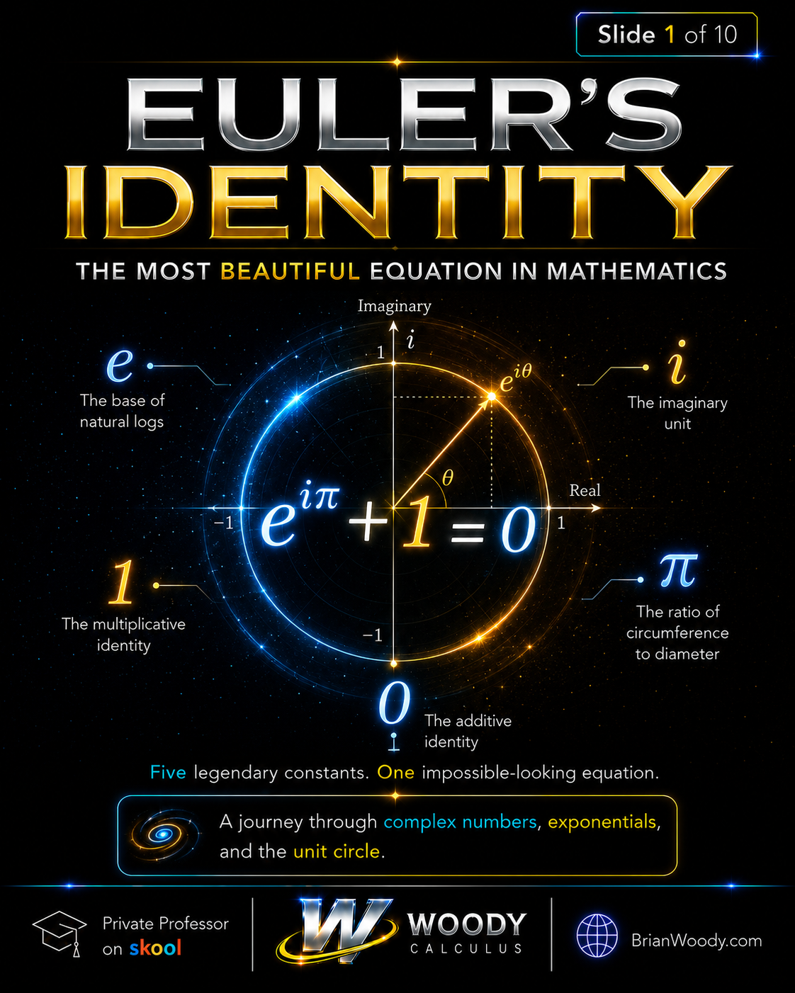
Euler’s Identity is often called the most beautiful equation in mathematics because it connects five legendary constants: e, i, π, 1, and 0. In this Woody Calculus visual lesson, we explain Euler’s formula, the complex plane, the unit circle, Taylor series, and why e^{iπ}+1=0 links algebra, geometry, analysis, waves, physics, and engineering.
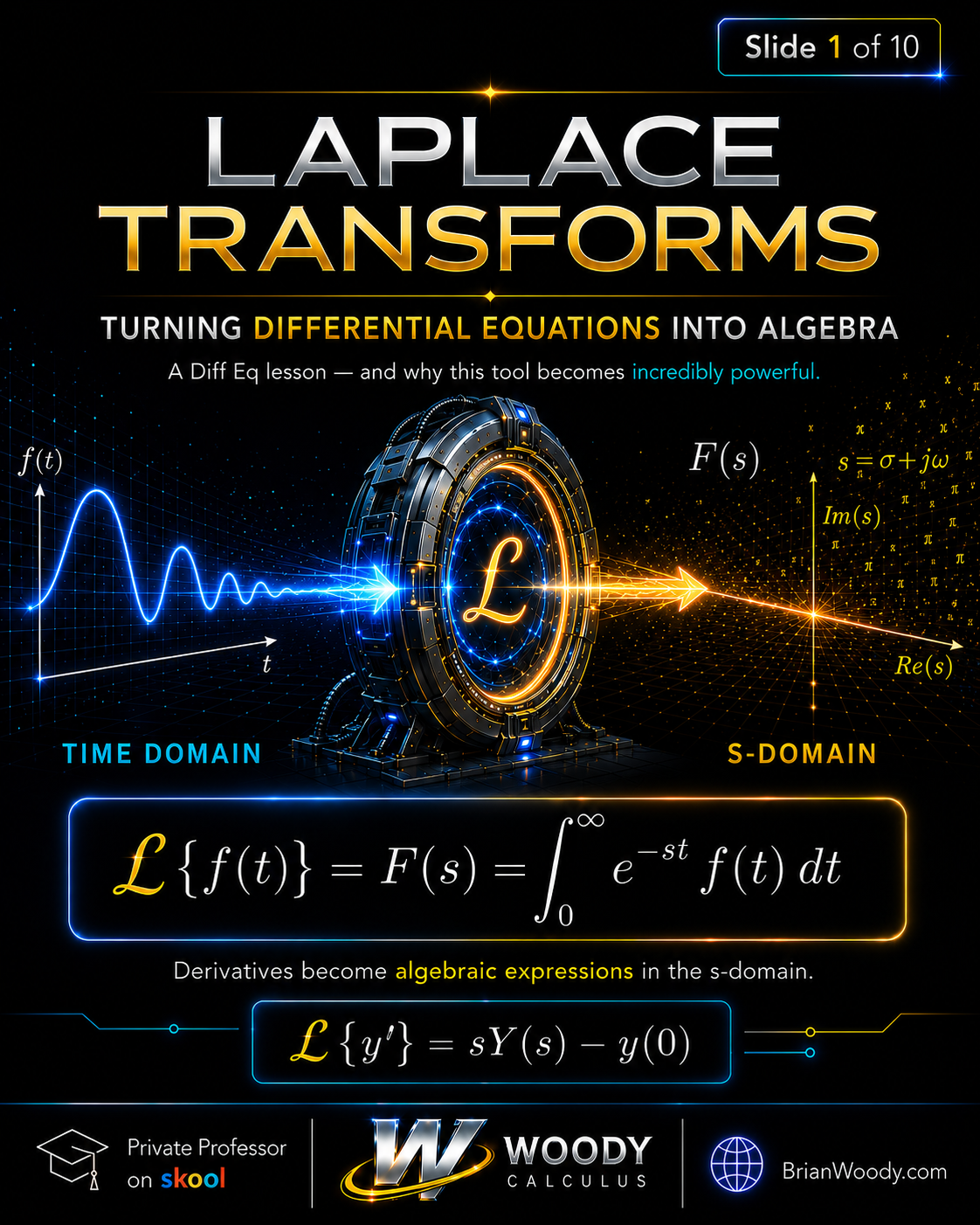
The Laplace Transform turns differential equations into algebra by moving time-domain functions into the s-domain. In this Woody Calculus visual lesson, learn the core formula, derivative rules, initial value problems, partial fractions, inverse Laplace transforms, unit step functions, and why Laplace transforms are so powerful for Differential Equations, engineering, circuits, and applied mathematics.