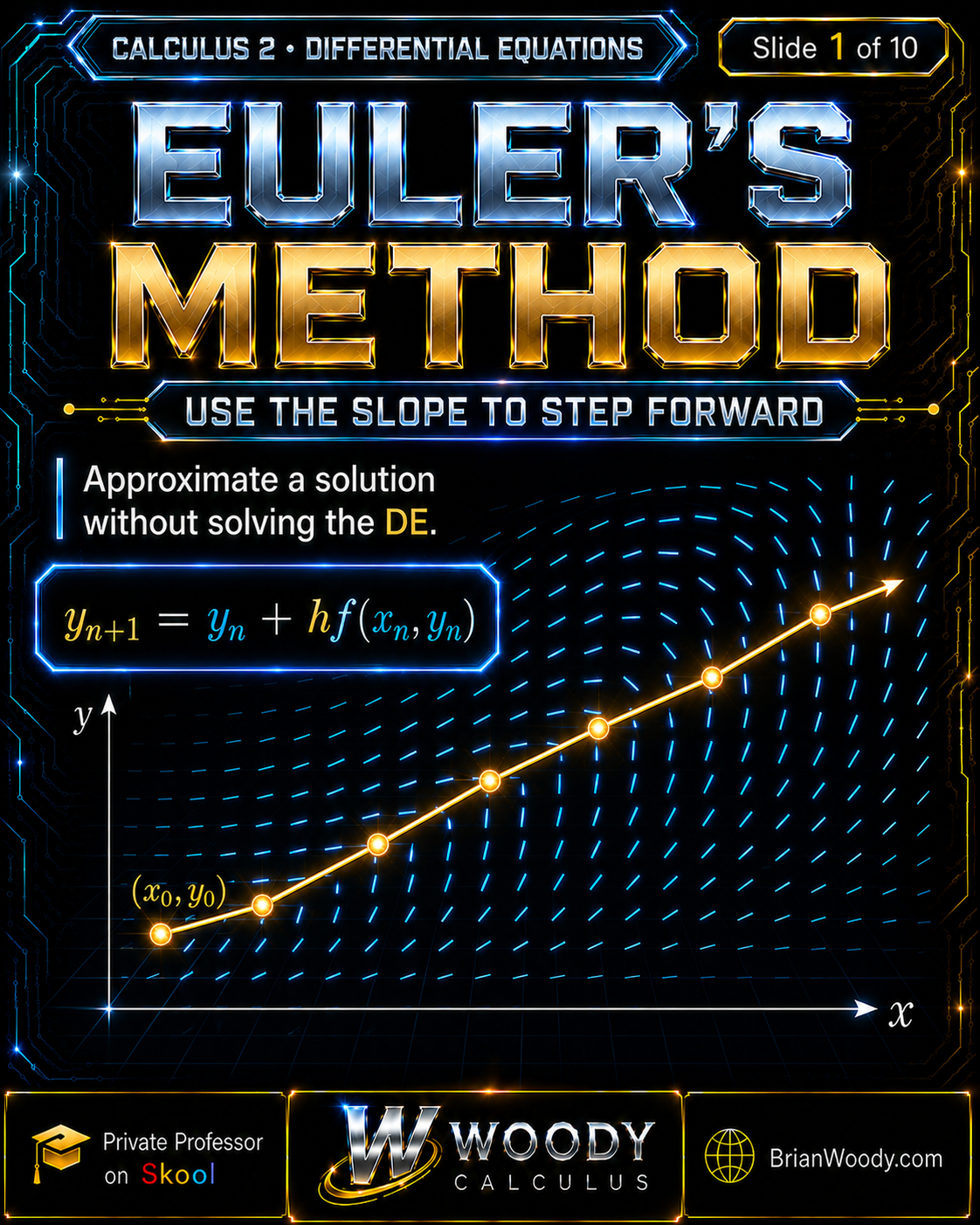
Euler’s method is a first-order numerical method that approximates the solution of an initial-value problem by using the differential equation’s slope at the current point to predict the next point.
Instead of solving the differential equation exactly, the method moves forward through a sequence of short tangent-line steps.
This matters because many differential equations either cannot be solved with elementary formulas or are easier to investigate numerically. Euler’s method is the foundational idea behind more advanced numerical methods: evaluate the slope, take a controlled step, and repeat.
What Is Euler’s Method?
Euler’s method approximates an unknown solution curve by replacing each short piece of the curve with a tangent-line step.
Suppose an initial-value problem has the form
y^{\prime}=f(x,y),
\qquad
y(x_0)=y_0.
\]
The initial condition provides the starting point \((x_0,y_0)\). The differential equation then provides the slope
m_0=f(x_0,y_0).
\]
Euler’s method follows that slope for a short horizontal distance \(h\). It then evaluates a new slope at the resulting approximation point and repeats the process.
Plain-language answer:
The equation tells you which direction to move, and the step size tells you how far to move before checking the slope again.
What Does the Differential Equation’s Slope Mean?
For a differential equation \(y^{\prime}=f(x,y)\), the number \(f(x,y)\) is the slope that a solution curve must have when it passes through \((x,y)\).
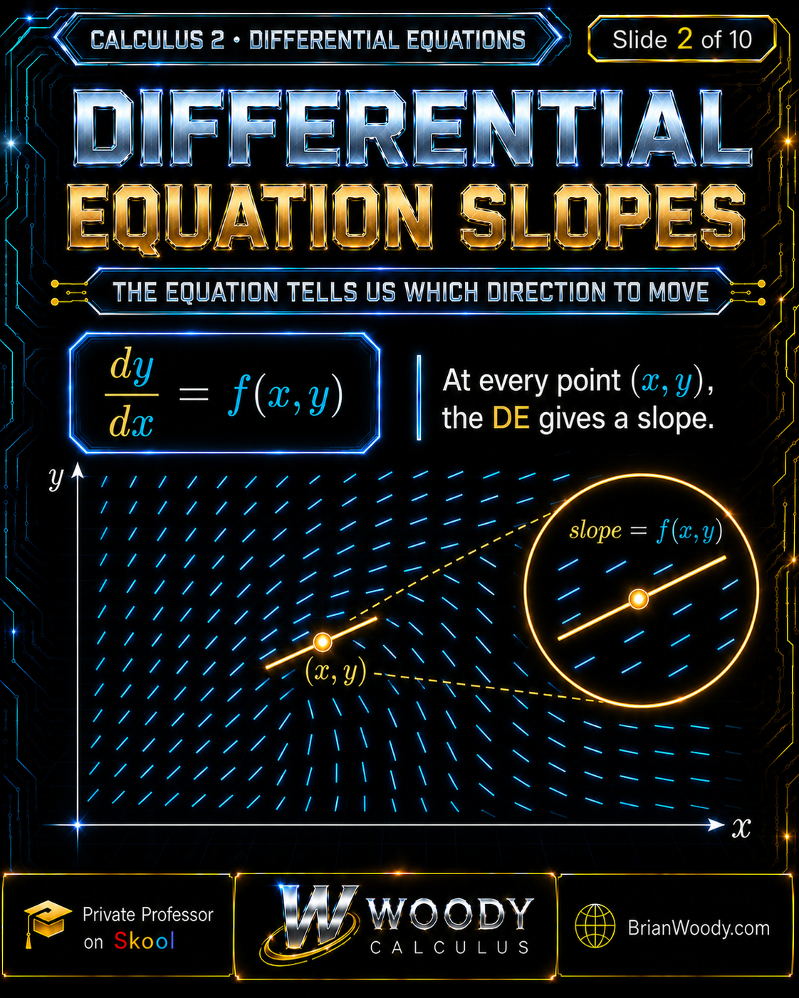
A slope field displays many short line segments. Each segment records the value of \(f(x,y)\) at its location. A genuine solution curve must move through the field while remaining tangent to these local directions.
Euler’s method does not follow the continuously changing curve itself. It freezes the slope at the left endpoint of each step and follows a straight segment until the next \(x\)-value.
What Is the Euler Method Formula?
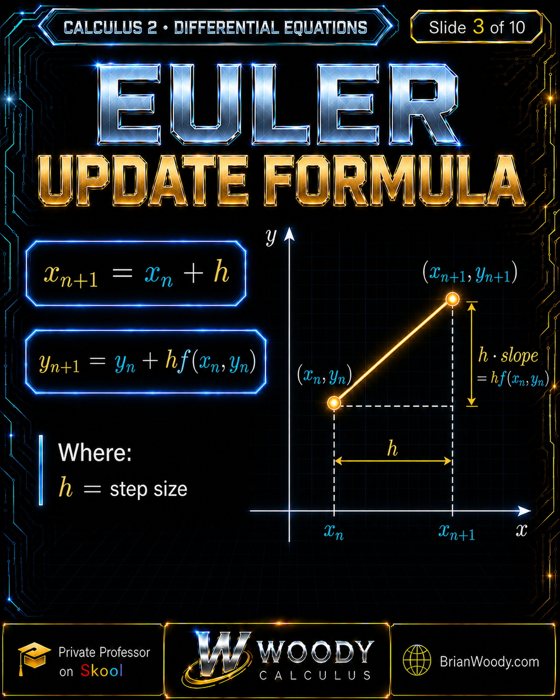
The Euler update advances \(x\) by \(h\) and advances \(y\) by \(h\) times the slope at the current point.
\boxed{x_{n+1}=x_n+h}
\]
\boxed{y_{n+1}=y_n+h f(x_n,y_n)}
\]
| Symbol | Meaning | Role in the method |
|---|---|---|
| \(x_n\) | Current input value | The left endpoint of the current step |
| \(y_n\) | Current approximate output | The current estimate of the solution |
| \(h\) | Step size | The horizontal distance between consecutive points |
| \(f(x_n,y_n)\) | Current slope | The differential equation evaluated at the current point |
| \(h f(x_n,y_n)\) | Predicted vertical change | The slope multiplied by the horizontal step |
Where Does the Formula Come From?
The tangent-line approximation near \(x_n\) is
y(x_n+h)\approx y(x_n)+h y^{\prime}(x_n).
\]
Because \(y^{\prime}=f(x,y)\), replace the derivative with the differential equation’s slope:
y(x_n+h)\approx y_n+h f(x_n,y_n).
\]
The approximation on the left becomes the next Euler value \(y_{n+1}\).
Plain-language answer:
Euler’s formula is the tangent-line formula used repeatedly instead of only once.
How Do You Complete One Euler Step?
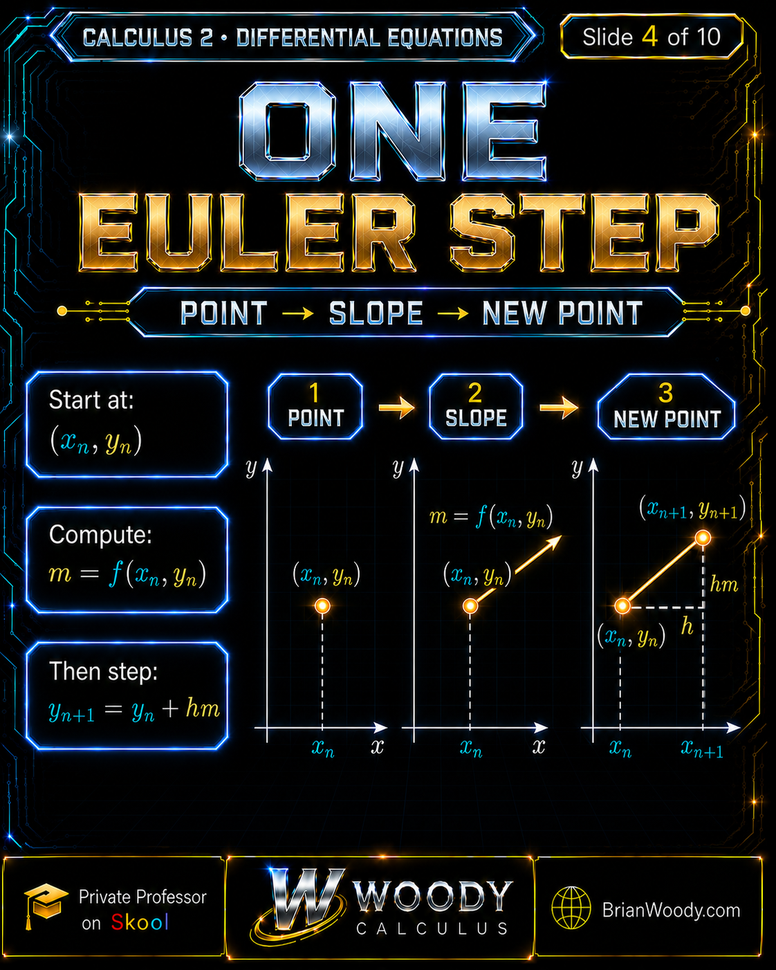
Record the current point, evaluate the current slope, multiply by the step size, and update both coordinates.
Step 1: Record the Current Point
(x_n,y_n).
\]
Step 2: Evaluate the Slope
m_n=f(x_n,y_n).
\]
Step 3: Update the Coordinates
x_{n+1}=x_n+h,
\qquad
y_{n+1}=y_n+h m_n.
\]
Step 4: Repeat at the New Point
The point \((x_{n+1},y_{n+1})\) becomes the current point for the next row of the table.
Formula memorization is required, but the equation’s structure chooses what must be substituted into the formula.
How Do You Build an Euler Method Table?
Create one row for each step and record \(x_n\), \(y_n\), the current slope, and the resulting next value.
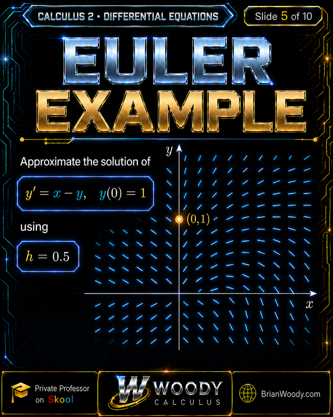
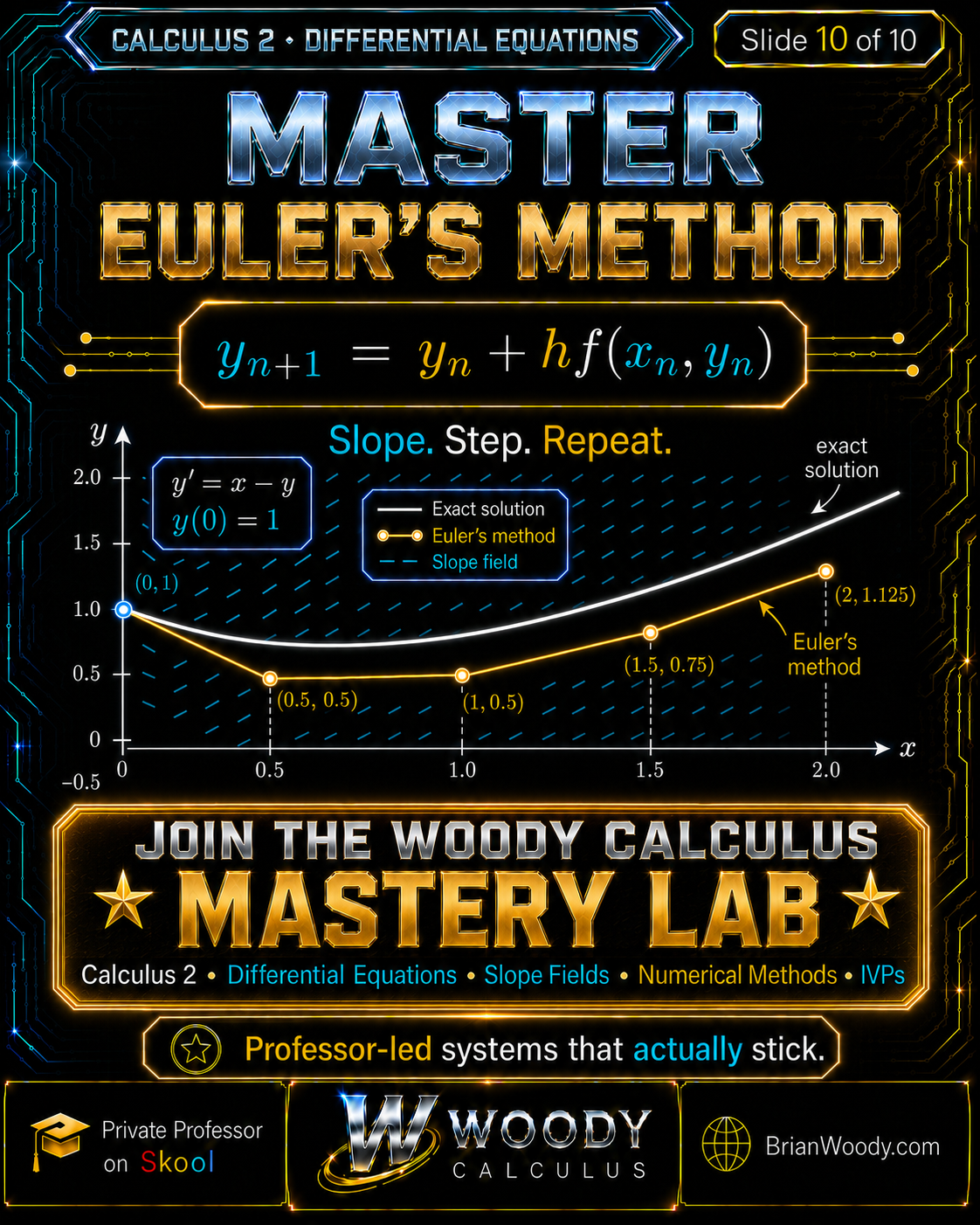
Approximate the solution of
y^{\prime}=x-y,
\qquad
y(0)=1,
\]
using the step size
h=0.5.
\]
First Euler Step
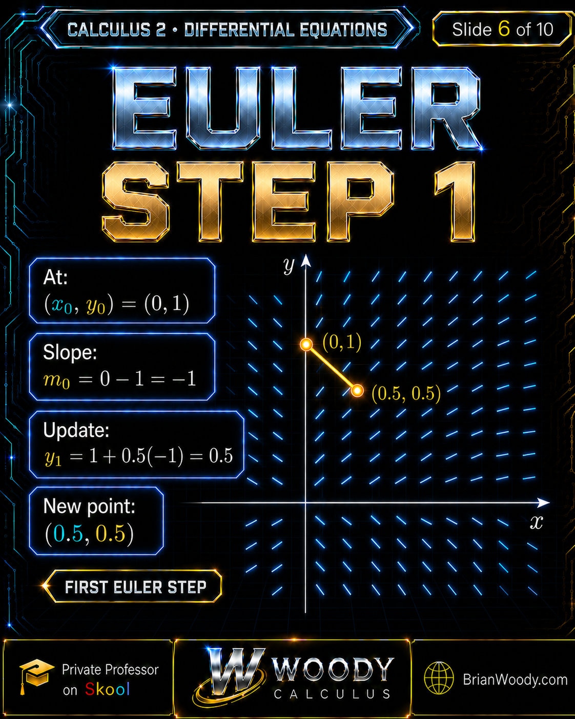
Begin with
(x_0,y_0)=(0,1).
\]
Evaluate the slope:
m_0=f(0,1)=0-1=-1.
\]
Update \(x\):
x_1=0+0.5=0.5.
\]
Update \(y\):
y_1=1+0.5(-1)=0.5.
\]
The first new point is
\boxed{(x_1,y_1)=(0.5,0.5)}.
\]
Complete Three-Step Table
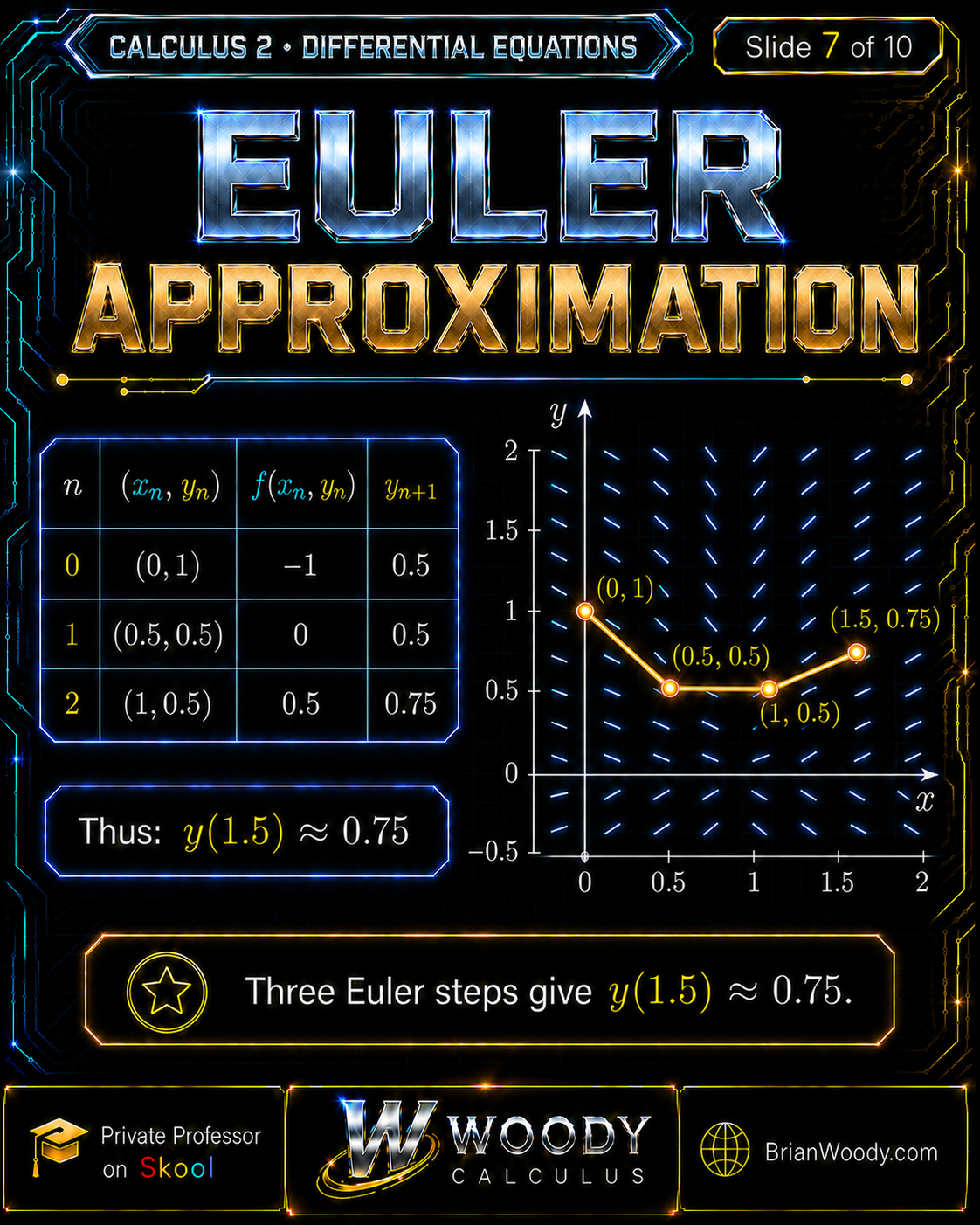
| \(n\) | \(x_n\) | \(y_n\) | \(f(x_n,y_n)=x_n-y_n\) | \(x_{n+1}\) | \(y_{n+1}=y_n+h f(x_n,y_n)\) |
|---|---|---|---|---|---|
| 0 | 0 | 1 | \(-1\) | 0.5 | 0.5 |
| 1 | 0.5 | 0.5 | 0 | 1 | 0.5 |
| 2 | 1 | 0.5 | 0.5 | 1.5 | 0.75 |
\boxed{y(1.5)\approx 0.75}
\]
Plain-language answer:
Every row begins with the point produced by the previous row. Never calculate all the slopes first and then try to update the values afterward.
How Can You Verify an Euler Approximation?
When an exact solution is available, solve the differential equation independently and compare its value with the Euler approximation.
The equation is a
first-order linear differential equation:
y^{\prime}+y=x.
\]
The integrating factor is
\mu(x)=e^{\int 1\,dx}=e^x.
\]
Multiplying the equation by \(e^x\) gives
e^x y^{\prime}+e^x y=xe^x.
\]
The left side is a product derivative:
\left(e^x y\right)^{\prime}=xe^x.
\]
Integrating gives
e^x y=e^x(x-1)+C.
\]
Therefore,
y=x-1+Ce^{-x}.
\]
Apply \(y(0)=1\):
1=-1+C,
\qquad
C=2.
\]
\boxed{y=x-1+2e^{-x}}
\]
Compare the Exact and Euler Values at \(x=1.5\)
y(1.5)
=
1.5-1+2e^{-1.5}
\approx
0.946260.
\]
Euler’s method with \(h=0.5\) gave \(0.75\). The absolute error is
\left|0.946260-0.75\right|
\approx
\boxed{0.196260}.
\]
Plain-language answer:
The Euler value is not intended to equal the exact value. The comparison measures how much accuracy was lost by following straight tangent segments instead of the continuously curving solution.
How Does Step Size Affect Accuracy?
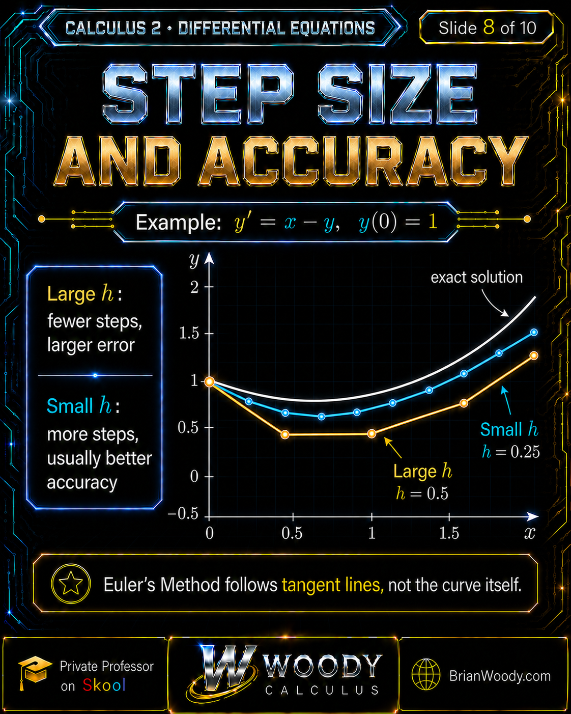
A smaller step size makes Euler’s method reevaluate the slope more frequently and usually reduces the accumulated approximation error.
For the same example, compare the approximations at \(x=2\).
| Method | Step size | Approximation at \(x=2\) | Absolute error |
|---|---|---|---|
| Euler | 0.5 | 1.125000 | 0.145671 |
| Euler | 0.25 | 1.200226 | 0.070445 |
| Exact solution | Not applicable | 1.270671 | 0 |
How Many Euler Steps Are Required?
To move from \(x_0\) to a target value \(b\) using a constant step size \(h\), the number of steps is
N=\frac{b-x_0}{h}.
\]
From \(x_0=0\) to \(b=1.5\) with \(h=0.5\):
N=\frac{1.5-0}{0.5}=3.
\]
Before beginning the table, verify that the proposed step size reaches the requested target. If the quotient is not an integer, the problem may require a different step size or a shorter final step.
What Is Euler’s Method Error?
Euler’s method has a one-step local truncation error of order \(h^2\) and, under standard smoothness and stability assumptions, a global error of order \(h\) over a fixed interval.
Taylor’s theorem gives
y(x_n+h)
=
y(x_n)
+
h y^{\prime}(x_n)
+
\frac{h^2}{2}y^{\prime\prime}(\xi_n)
\]
for some \(\xi_n\) between \(x_n\) and \(x_n+h\). Euler’s method keeps the first two terms and discards the curvature term.
\text{one-step local truncation error}
=
O(h^2).
\]
A fixed interval contains approximately \(1/h\) steps. The accumulated error therefore ordinarily satisfies
\text{global error}
=
O(h).
\]
This is why Euler’s method is called a first-order method. Halving the step size should approximately halve the global error once the calculation is in the expected asymptotic regime.
Why Does Euler’s Method Drift Away from the Exact Solution?
If you are wondering why Euler’s method diverges from the exact solution over time, the reason is that every step follows one frozen tangent line while the true slope keeps changing. Each small curvature error becomes part of the next starting value, so the errors accumulate from step to step.
Plain-language answer:
Each individual step makes a small curvature error. Many small errors accumulate, so the final error usually decreases in direct proportion to the step size.
What Are the Most Common Euler Method Mistakes?
Mistake 1: Evaluating the Slope at the New Point
Forward Euler uses the known current point:
f(x_n,y_n).
\]
Using \(f(x_{n+1},y_{n+1})\) defines a different method—implicit or backward Euler—and usually creates an equation that must be solved for \(y_{n+1}\). If your table suddenly becomes algebraically implicit, check where you evaluated the slope.
Mistake 2: Forgetting to Multiply the Slope by \(h\)
The slope is not the vertical change. The vertical change is
\Delta y=h f(x_n,y_n).
\]
If the approximation jumps too far vertically—especially when \(0<h<1\)—check whether you forgot the factor \(h\).
Mistake 3: Forgetting the \(x\)-Update
Every row requires both updates:
x_{n+1}=x_n+h,
\qquad
y_{n+1}=y_n+h f(x_n,y_n).
\]
If the final row does not land on the requested input value, inspect the \(x\)-column first.
Mistake 4: Using the Wrong Row’s Values
After computing \((x_{n+1},y_{n+1})\), that point becomes the input for the next slope. Do not reuse \((x_n,y_n)\). Repeated or suspiciously unchanged slope values often reveal this error.
Mistake 5: Rounding Too Early
Keep exact fractions or several decimal places throughout the table. Round only the requested final approximation unless the problem explicitly gives another instruction. If the last few rows drift unexpectedly, compare them with an unrounded calculation.
Mistake 6: Taking the Wrong Number of Steps
Calculate
N=\frac{b-x_0}{h}
\]
before beginning. If your answer is attached to the wrong \(x\)-value, you probably stopped one row too early or continued one row too far.
Mistake 7: Reporting an Approximation as an Exact Equality
Use the approximation symbol:
y(1.5)\approx0.75,
\]
not \(y(1.5)=0.75\), unless the value has independently been proven exact.
Mistake 8: Assuming a Smaller Step Removes Every Numerical Problem
A smaller step may reduce truncation error, but it does not automatically fix instability, incorrect arithmetic, a discontinuous slope function, or a method that is poorly suited to the problem. If values explode or oscillate unexpectedly, check the equation, arithmetic, and stability—not only the step size.
What Checklist Should You Use on an Exam?
Use the same organized sequence on every Euler problem so that no slope, coordinate, or step is lost.
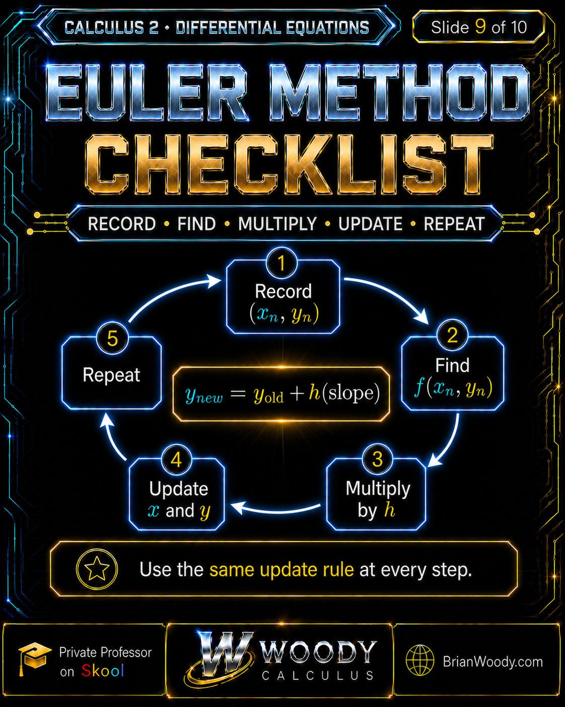
- Classify the problem: Confirm that a forward Euler approximation is requested.
- Write the formula from memory: Include both the \(x\)- and \(y\)-updates.
- Identify the data: Record \(f(x,y)\), \((x_0,y_0)\), \(h\), and the target \(x\)-value.
- Determine the number of steps: Calculate \(N=(b-x_0)/h\).
- Evaluate the slope: Substitute the current \(x_n\) and \(y_n\) into \(f\).
- Multiply by \(h\): Calculate the predicted vertical change.
- Update both coordinates: Calculate \(x_{n+1}\) and \(y_{n+1}\).
- Repeat with the new point: Never reuse the previous row accidentally.
- Verify the target: Confirm that the final \(x_n\) is the requested input.
- Check the direction: Compare the sign of each slope with the plotted movement.
- Compare step sizes when possible: Recompute with \(h/2\).
- Use an exact solution when available: Calculate the absolute error.
- Rewrite the complete solution from memory: Rebuild the table from a blank page.
- Say each step out loud: Point, slope, multiply, update, repeat.
Reading a completed Euler table is not enough. Rebuild the setup from a blank page until the method becomes automatic.
Euler’s Method FAQ
What is Euler’s method?
Euler’s method is an explicit first-order numerical method that approximates the solution of an initial-value problem by using the slope at the current point to predict the next point.
What formula is used for Euler’s method?
The updates are \(x_{n+1}=x_n+h\) and \(y_{n+1}=y_n+h f(x_n,y_n)\), where \(h\) is the step size and \(f(x_n,y_n)\) is the current slope.
How do you determine the number of Euler steps?
For a constant step size, use \(N=(b-x_0)/h\), where \(x_0\) is the starting input and \(b\) is the target input. Confirm that the quotient is an integer unless a shorter final step is allowed.
Does a smaller step size always make Euler’s method more accurate?
A smaller step size usually improves accuracy for a smooth problem and a stable computation because the slope is reevaluated more frequently. It also requires more work and does not automatically eliminate instability or floating-point error.
What is the difference between a slope field and Euler’s method?
A slope field displays the slope assigned by the differential equation at many points. Euler’s method selects slopes from that field and uses them to construct a polygonal numerical approximation beginning at the initial condition.
Is Euler’s method an exact method?
Euler’s method is generally approximate. It is exact only in special situations, such as when the relevant solution is linear over the interval and the tangent-line step reproduces the curve exactly.
What is the order of error in Euler’s method?
The one-step local truncation error is ordinarily of order \(h^2\), and the accumulated global error over a fixed interval is ordinarily of order \(h\) under standard smoothness and stability assumptions.
Can Euler’s method be used when the exact solution is unknown?
Yes. Approximating solutions when an exact formula is unavailable or inconvenient is one of the main purposes of Euler’s method. Accuracy can be assessed by reducing the step size or comparing with a more accurate numerical method.
Why does Euler’s method drift away from the exact solution?
Euler’s method follows a frozen tangent slope across each step while the true solution’s slope changes continuously. The resulting curvature error becomes part of the next starting value, so the errors accumulate.
How can you tell whether an Euler table is wrong?
Check that every row uses the current point, that the slope is multiplied by \(h\), that both coordinates are updated, that the final row reaches the requested input, and that each plotted segment moves in the direction indicated by its slope.
How Do You Master Euler’s Method?
Master Euler’s method by memorizing the two updates and rebuilding complete tables until the sequence becomes automatic.
Private Differential Equations Instruction
The
Woody Calculus Mastery Lab
is the required first step for students seeking structured help with Euler’s method, slope fields, initial-value problems, separable equations, linear equations, systems, and exam preparation.
Limited
private instruction
is selective, normally requires weekly sessions, requires active Mastery Lab enrollment first, and is not guaranteed. Students and parents may use the
Woody Calculus contact page
for questions about the appropriate starting point.
University Calculus and Differential Equations Help
Woody Calculus provides professor-led online support for students taking Calculus 2, Differential Equations, Linear Algebra, and related university mathematics courses.
Visit the
university mathematics help hub
to explore additional university pages.
Woody Calculus Reviews
★★★★★
Read
Woody Calculus 5-star Google reviews
and view
Brian M. Woody’s 5.0 RateMyProfessors rating.
Students ready to build a more reliable system can begin with the
Woody Calculus Mastery Lab on Skool.