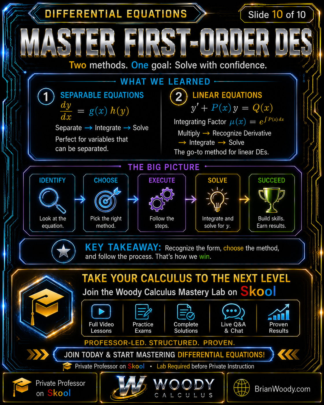
A first-order differential equation is separable when its \(x\)-terms and \(y\)-terms can be placed on opposite sides, and it is linear when it can be written in the form \(y^{\prime}+P(x)y=Q(x)\).
That distinction determines the method:
- Separable equation: separate the variables, integrate both sides, and solve for \(y\) when possible.
- First-order linear equation: put the equation in standard form, find an integrating factor, create a product derivative, integrate, and solve.
The most important habit in Differential Equations is therefore not immediate computation.
Classify the equation before choosing the method.
Students frequently lose time because they begin manipulating an equation before identifying its structure. They may attempt separation on an equation that cannot be separated, or use an integrating factor when separation would solve the problem in three lines.
This Woody Calculus lesson develops a complete decision system for two of the most common first-order ordinary differential equation methods:
- separation of variables,
- the first-order linear integrating-factor method.
It also explains what to do when an equation belongs to both categories, how to avoid losing equilibrium solutions, why the integrating factor creates a product derivative, how to use initial conditions, and how to verify a final answer.
Published: .
Last updated: .
Estimated read time: 20–24 minutes.
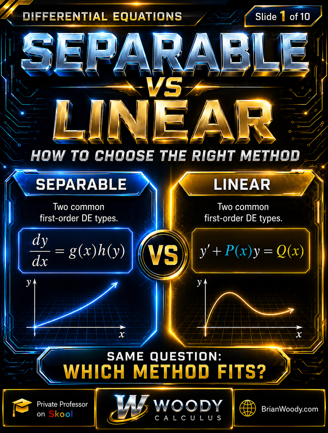
What Is the Difference Between Separable and Linear Differential Equations?
A separable equation is identified by whether the variables can be separated, while a linear equation is identified by the powers and coefficients of \(y\) and \(y^{\prime}\).
| Feature | Separable Equation | First-Order Linear Equation |
|---|---|---|
| Typical Form | \(\frac{dy}{dx}=g(x)h(y)\) | \(y^{\prime}+P(x)y=Q(x)\) |
| Main Test | Can all \(y\)-terms go with \(dy\) and all \(x\)-terms go with \(dx\)? | Do \(y\) and \(y^{\prime}\) appear only to the first power, with coefficients depending only on \(x\)? |
| Main Tool | Separation of variables | Integrating factor |
| Core Action | Separate and integrate | Create and integrate a product derivative |
| Can It Be Nonlinear? | Yes | No, it is linear in \(y\) |
Plain-language answer: separability is about moving variables to opposite sides; linearity is about the equation’s algebraic structure in \(y\) and \(y^{\prime}\).
Why Should You Classify a Differential Equation Before Solving?
Classification identifies the solution method and prevents unnecessary algebra.
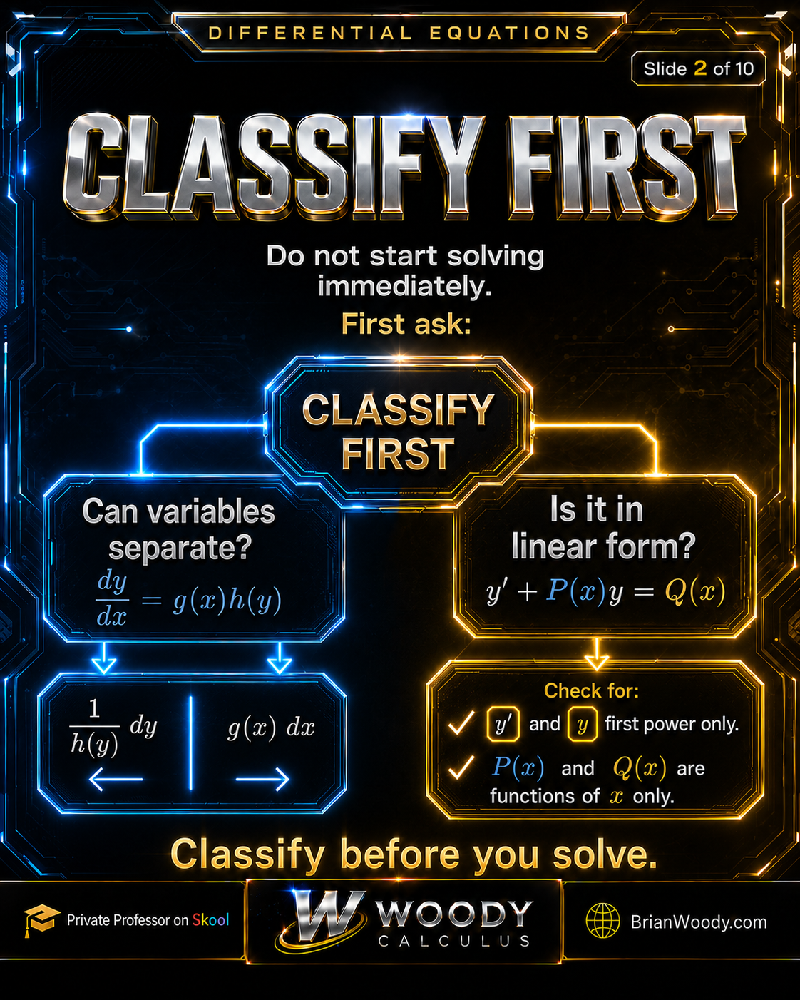
Before differentiating, integrating, substituting, or rearranging extensively, ask two questions:
- Can the variables be separated?
- Can the equation be written in first-order linear form?
The separable test asks whether the equation can become:
\frac{1}{h(y)}\,dy=g(x)\,dx.
\]
The linear test asks whether the equation can become:
y^{\prime}+P(x)y=Q(x).
\]
Do not decide based only on how the original equation looks. Simplify and rearrange enough to reveal its true form.
Identify the structure. Choose the method. Then execute the steps.
What Is a Separable Differential Equation?
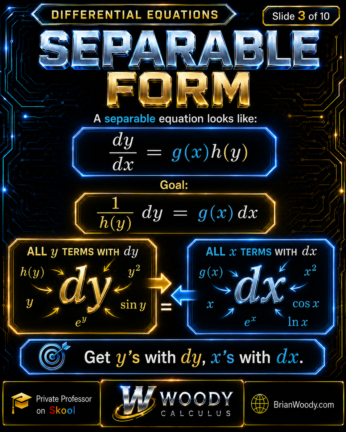
A first-order differential equation is separable if it can be rewritten with every \(y\)-dependent factor beside \(dy\) and every \(x\)-dependent factor beside \(dx\).
A common separable form is:
\boxed{
\frac{dy}{dx}=g(x)h(y).
}
\]
When \(h(y)\ne0\), divide by \(h(y)\) and multiply by \(dx\):
\boxed{
\frac{1}{h(y)}\,dy=g(x)\,dx.
}
\]
The left side now contains only \(y\) and \(dy\). The right side contains only \(x\) and \(dx\).
Examples of separable equations include:
y^{\prime}=xy^2,
\]
y^{\prime}=e^x(1-y),
\]
y^{\prime}=y\cos x.
\]
How to Solve a Separable Differential Equation
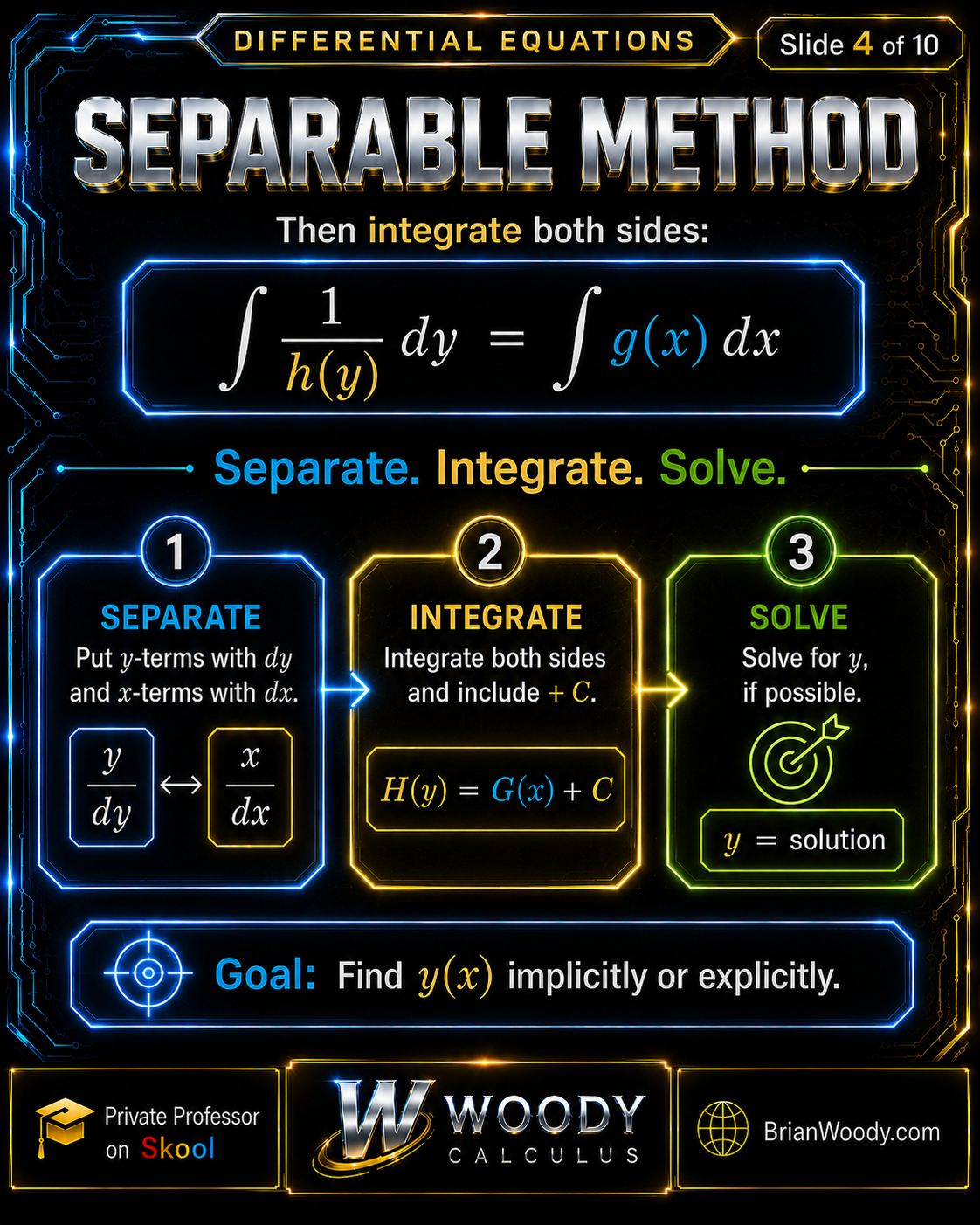
The separable method has three main stages: separate, integrate, and solve.
Step 1: Separate the Variables
Starting with:
\frac{dy}{dx}=g(x)h(y),
\]
rewrite as:
\frac{1}{h(y)}\,dy=g(x)\,dx.
\]
Step 2: Integrate Both Sides
\int\frac{1}{h(y)}\,dy
=
\int g(x)\,dx.
\]
Write the constant of integration once:
H(y)=G(x)+C.
\]
Step 3: Solve for \(y\), If Possible
Some separable equations produce an explicit solution:
y=f(x).
\]
Others are best left in implicit form:
F(x,y)=C.
\]
Both forms can be valid.
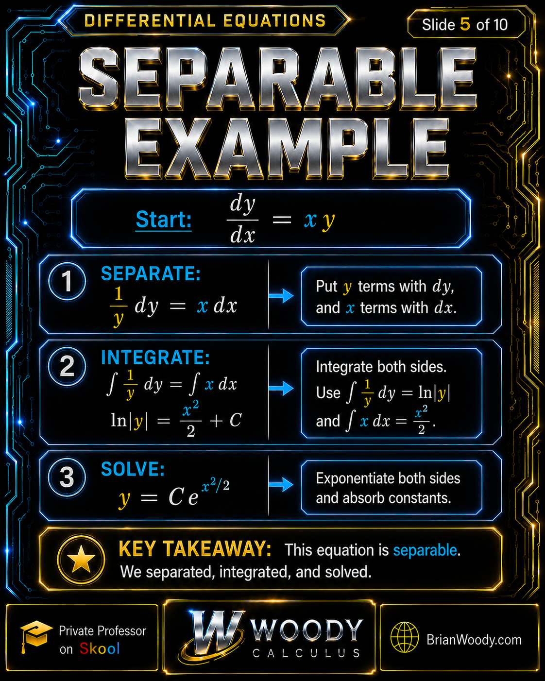
Separable Differential Equation Example: Solve \(\frac{dy}{dx}=xy\)
The equation is separable because its right side is a product of a function of \(x\) and a function of \(y\).
\frac{dy}{dx}=xy.
\]
Step 1: Check for Equilibrium Solutions
Since the \(y\)-factor is \(h(y)=y\), the value \(y=0\) makes the right side zero.
Therefore:
y=0
\]
is a constant solution.
Step 2: Separate for \(y\ne0\)
\frac{1}{y}\,dy=x\,dx.
\]
Step 3: Integrate Both Sides
\int\frac{1}{y}\,dy
=
\int x\,dx.
\]
\ln|y|=\frac{x^2}{2}+C.
\]
The absolute value is required because:
\int\frac{1}{y}\,dy=\ln|y|+C.
\]
Step 4: Exponentiate and Absorb the Constant
|y|=e^C e^{x^2/2}.
\]
Absorb the sign and positive constant into one arbitrary constant \(C\):
\boxed{
y=Ce^{x^2/2}.
}
\]
Allowing \(C=0\) includes the equilibrium solution \(y=0\). Thus the complete solution family is:
\boxed{
y=Ce^{x^2/2},
\qquad C\in\mathbb{R}.
}
\]
Step 5: Verify
Differentiate:
y^{\prime}
=
Cxe^{x^2/2}.
\]
Since \(y=Ce^{x^2/2}\):
y^{\prime}=xy.
\]
Plain-language answer: the complete family of solutions is \(y=Ce^{x^2/2}\).
What Is a First-Order Linear Differential Equation?
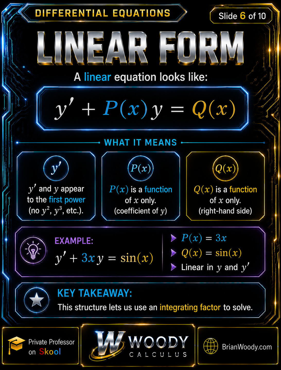
A first-order differential equation is linear when it can be written as \(y^{\prime}+P(x)y=Q(x)\).
\boxed{
y^{\prime}+P(x)y=Q(x).
}
\]
The requirements are:
- \(y^{\prime}\) appears to the first power,
- \(y\) appears to the first power,
- \(y\) and \(y^{\prime}\) are not multiplied together,
- there are no nonlinear expressions such as \(y^2\), \(\sin y\), or \(e^y\),
- \(P(x)\) and \(Q(x)\) depend only on \(x\).
For example:
y^{\prime}+3xy=\sin x
\]
is linear because:
P(x)=3x,
\qquad
Q(x)=\sin x.
\]
Normalize the Equation First
If the equation begins as:
a(x)y^{\prime}+b(x)y=c(x),
\]
divide by \(a(x)\) on an interval where \(a(x)\ne0\):
y^{\prime}
+
\frac{b(x)}{a(x)}y
=
\frac{c(x)}{a(x)}.
\]
Only after normalization should you identify \(P(x)\) and \(Q(x)\).
Why Does the Integrating Factor Method Work?
The integrating factor is chosen so that the left side of the linear equation becomes the derivative of a product.
Begin with:
y^{\prime}+P(x)y=Q(x).
\]
Define the integrating factor:
\boxed{
\mu(x)=e^{\int P(x)\,dx}.
}
\]
Because:
\mu^{\prime}(x)=P(x)\mu(x),
\]
multiplying every term by \(\mu(x)\) gives:
\mu y^{\prime}+\mu P(x)y=\mu Q(x).
\]
The product rule says:
\frac{d}{dx}[\mu y]
=
\mu y^{\prime}+\mu^{\prime}y.
\]
Since \(\mu^{\prime}=P\mu\):
\frac{d}{dx}[\mu y]
=
\mu y^{\prime}+\mu P(x)y.
\]
Therefore the differential equation becomes:
\boxed{
\frac{d}{dx}[\mu(x)y]
=
\mu(x)Q(x).
}
\]
Integrate:
\mu(x)y
=
\int\mu(x)Q(x)\,dx+C.
\]
Solve for \(y\):
\boxed{
y=
\frac{1}{\mu(x)}
\left[
\int\mu(x)Q(x)\,dx+C
\right].
}
\]
Plain-language answer: the integrating factor works because it converts two separate terms into one product derivative.
![Integrating-factor method showing μ(x) = e^(∫P(x)dx) and the product derivative d/dx[μ(x)y] = μ(x)Q(x), from Woody Calculus.](https://k3p6r8v3.delivery.rocketcdn.me/wp-content/uploads/2026/07/Separable-vs-Linear-Slide-7.png "Integrating Factor Method")
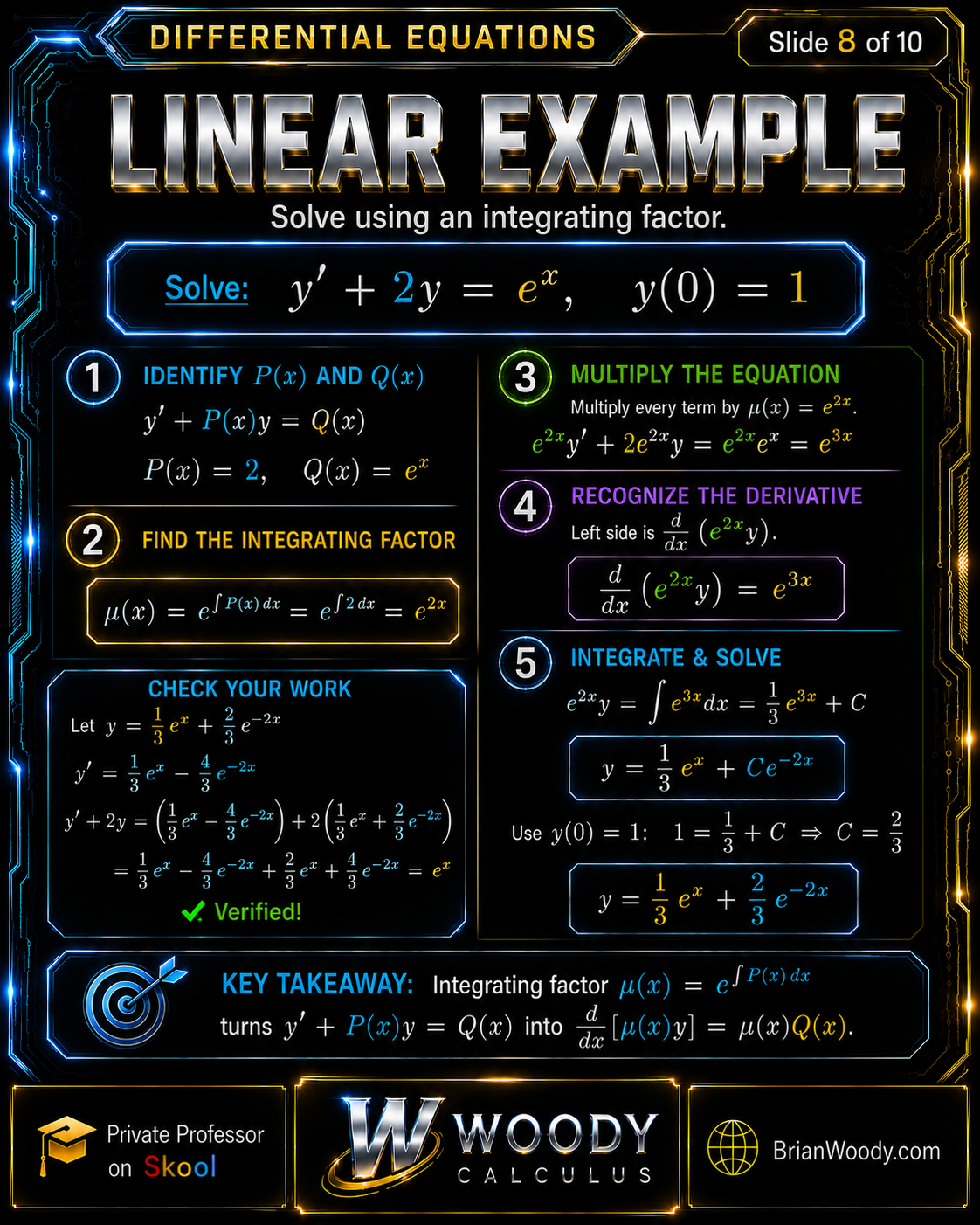
First-Order Linear Example: Solve \(y^{\prime}+2y=e^x,\ y(0)=1\)
This equation is already in standard linear form with \(P(x)=2\) and \(Q(x)=e^x\).
y^{\prime}+2y=e^x,
\qquad
y(0)=1.
\]
Step 1: Identify \(P(x)\) and \(Q(x)\)
P(x)=2,
\qquad
Q(x)=e^x.
\]
Step 2: Find the Integrating Factor
\mu(x)
=
e^{\int2\,dx}
=
e^{2x}.
\]
Step 3: Multiply Every Term by \(e^{2x}\)
e^{2x}y^{\prime}
+
2e^{2x}y
=
e^{3x}.
\]
Step 4: Recognize the Product Derivative
\frac{d}{dx}\left(e^{2x}y\right)
=
e^{3x}.
\]
Step 5: Integrate
e^{2x}y
=
\int e^{3x}\,dx
=
\frac13e^{3x}+C.
\]
Step 6: Solve for \(y\)
y
=
\frac13e^x
+
Ce^{-2x}.
\]
Step 7: Apply the Initial Condition
1
=
\frac13+C
\quad\Longrightarrow\quad
C=\frac23.
\]
Final answer:
\boxed{
y=
\frac13e^x
+
\frac23e^{-2x}.
}
\]
Step 8: Verify
y^{\prime}
=
\frac13e^x
–
\frac43e^{-2x}.
\]
Then:
\begin{aligned}
y^{\prime}+2y
&=
\left(
\frac13e^x-\frac43e^{-2x}
\right)
+
2\left(
\frac13e^x+\frac23e^{-2x}
\right)\\
&=
e^x.
\end{aligned}
\]
Also:
y(0)=\frac13+\frac23=1.
\]
Plain-language answer: the unique solution satisfying the initial condition is \(y=\frac13e^x+\frac23e^{-2x}\).
Separable vs. Linear Differential Equations Decision Table
Test separability and linearity independently because an equation may satisfy one test, both tests, or neither test.
| Differential Equation | Separable? | Linear? | Best Method |
|---|---|---|---|
| \(y^{\prime}=xy^2\) | Yes | No, because of \(y^2\) | Separation of variables |
| \(y^{\prime}+3y=e^x\) | Not directly | Yes | Integrating factor |
| \(y^{\prime}+2y=0\) | Yes | Yes | Usually separation |
| \(y^{\prime}=x(1-y)\) | Yes | Yes, since \(y^{\prime}+xy=x\) | Choose the cleaner method |
| \(y^{\prime}=x+y^2\) | No | No | Another method is needed |
The fastest classification rule is:
- Try to factor or rearrange the equation into an \(x\)-only factor times a \(y\)-only factor.
- Independently test whether it fits \(y^{\prime}+P(x)y=Q(x)\).
- If both tests work, choose the shorter method.
Can a Differential Equation Be Both Separable and Linear?
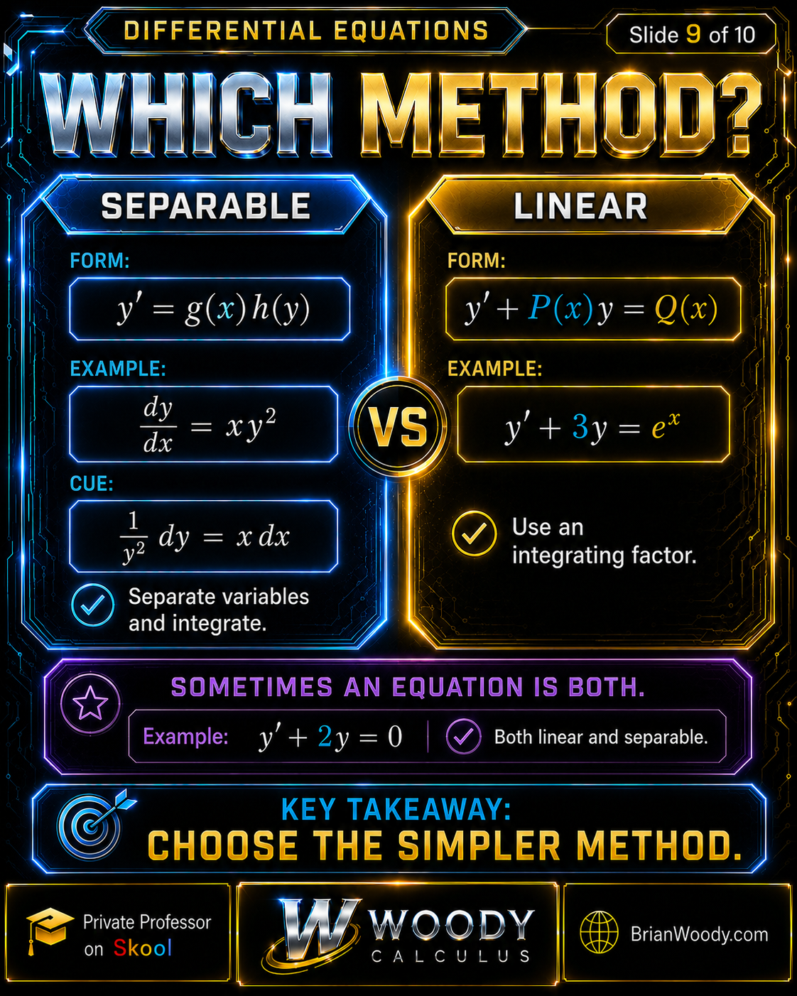
Yes. A first-order equation can satisfy both classifications.
Consider:
y^{\prime}+2y=0.
\]
It is linear because it has the form:
y^{\prime}+P(x)y=Q(x),
\qquad
P(x)=2,
\quad
Q(x)=0.
\]
It is also separable:
\frac{dy}{dx}=-2y.
\]
\frac{1}{y}\,dy=-2\,dx.
\]
Integrate:
\ln|y|=-2x+C.
\]
Exponentiating and absorbing constants gives:
\boxed{
y=Ce^{-2x}.
}
\]
Separation is shorter here, so it is the natural choice.
A valid method is good. The simplest valid method is better.
What If a Differential Equation Is Neither Separable Nor Linear?
If neither classification works, do not force one of these methods onto the equation.
Other first-order differential equation types include:
- exact equations,
- Bernoulli equations,
- homogeneous substitution equations,
- autonomous equations,
- equations requiring a special substitution,
- equations that do not have an elementary closed-form solution.
For example:
y^{\prime}=x+y^2
\]
is not separable because the right side is a sum that cannot be factored into an \(x\)-only function times a \(y\)-only function. It is not linear because of \(y^2\).
Classification still helps because it tells you which methods not to use.
How Do You Use an Initial Condition?
An initial condition determines the arbitrary constant in the general solution.
A first-order initial value problem usually has the form:
\text{differential equation},
\qquad
y(x_0)=y_0.
\]
The standard process is:
- Find the general solution containing \(C\).
- Substitute \(x=x_0\) and \(y=y_0\).
- Solve for \(C\).
- Write the particular solution.
- Verify the differential equation and initial condition.
In some separable equations, it is convenient to apply the initial condition while the solution is still implicit. That is acceptable as long as the algebra is consistent and the final interval of validity is considered.
How Do You Verify a Differential Equation Solution?
Differentiate the proposed solution, substitute it into the original equation, and check every initial or boundary condition.
A complete verification includes:
- Compute \(y^{\prime}\).
- Substitute \(y\) and \(y^{\prime}\) into the original differential equation.
- Simplify both sides independently.
- Confirm they are equal.
- Check the initial condition.
- State the interval on which the solution is defined.
Verification is especially important after exponentiating, dividing by expressions containing \(y\), or absorbing constants.
Common Separable and Linear Differential Equation Mistakes
Mistake 1: Solving Before Classifying
Identify the equation type before beginning the method.
Mistake 2: Calling Every Equation \(y^{\prime}=f(x,y)\) Separable
The right side must be factorable or rearrangeable into an \(x\)-only part and a \(y\)-only part.
Mistake 3: Forgetting Equilibrium Solutions
Dividing by \(h(y)\) may exclude constant solutions satisfying \(h(y)=0\).
Mistake 4: Writing \(\ln y\) Instead of \(\ln|y|\)
\int\frac1y\,dy=\ln|y|+C.
\]
Mistake 5: Forgetting the Constant of Integration
Write \(+C\) after integrating the two sides.
Mistake 6: Identifying \(P(x)\) Before Normalizing
The coefficient of \(y^{\prime}\) must first be made equal to \(1\).
Mistake 7: Using the Wrong Sign in the Integrating Factor
The sign of \(P(x)\) must be carried into the integrating-factor formula.
For example, in:
y^{\prime}-2y=e^x,
\]
the coefficient is:
P(x)=-2,
\]
not \(2\). Therefore:
\boxed{
\mu(x)
=
e^{\int-2\,dx}
=
e^{-2x}.
}
\]
Mistake 8: Multiplying Only Part of the Linear Equation by \(\mu\)
Every term on both sides must be multiplied by the integrating factor.
Mistake 9: Failing to Recognize the Product Derivative
After multiplying by \(\mu\), rewrite the complete left side as \(\frac{d}{dx}[\mu y]\).
Mistake 10: Using a More Complicated Method Than Necessary
If an equation is both linear and separable, select the shorter method.
The Woody Calculus First-Order Differential Equations Checklist
- Simplify the equation enough to reveal its structure.
- Check whether the variables can separate.
- Check whether the equation is linear in \(y\) and \(y^{\prime}\).
- If both methods apply, choose the simpler one.
- For separable equations, check equilibrium solutions before dividing.
- Separate all \(y\)-terms with \(dy\) and all \(x\)-terms with \(dx\).
- For linear equations, normalize before identifying \(P(x)\).
- Compute \(\mu(x)=e^{\int P(x)\,dx}\).
- Multiply every term by \(\mu(x)\).
- Recognize the product derivative.
- Integrate and include \(+C\).
- Apply the initial condition.
- Verify the equation and the initial condition.
- Rewrite the complete solution from memory and say each step out loud.
Formula memorization matters, but the equation’s structure chooses the formula. Classify first. Choose second. Execute third. Verify last.
Separable vs. Linear Differential Equations FAQ
What is a separable differential equation?
A separable differential equation can be rewritten with all \(y\)-dependent terms beside \(dy\) and all \(x\)-dependent terms beside \(dx\).
What is a first-order linear differential equation?
A first-order linear differential equation can be written as \(y^{\prime}+P(x)y=Q(x)\), where \(P\) and \(Q\) depend only on \(x\).
How do I tell whether an equation is separable or linear?
Test whether the variables can be separated into \(M(y)\,dy=N(x)\,dx\), and independently test whether the equation can be written as \(y^{\prime}+P(x)y=Q(x)\).
Can a differential equation be both separable and linear?
Yes. For example, \(y^{\prime}+2y=0\) is linear and can also be rewritten as \(\frac1y\,dy=-2\,dx\).
Which method should I use if an equation is both?
Use the valid method that produces the cleanest and shortest solution. Separation is often simpler for homogeneous first-order linear equations.
What is separation of variables?
Separation of variables rewrites a differential equation so the \(y\)-terms and \(dy\) are on one side and the \(x\)-terms and \(dx\) are on the other, after which both sides are integrated.
What is an integrating factor?
For \(y^{\prime}+P(x)y=Q(x)\), the integrating factor is \(\mu(x)=e^{\int P(x)\,dx}\).
Why does the integrating factor work?
It makes the left side equal to the product derivative \(\frac{d}{dx}[\mu(x)y]\), allowing the equation to be integrated directly.
Why must a linear equation be normalized first?
The integrating-factor formula assumes the coefficient of \(y^{\prime}\) is \(1\). Divide by the original coefficient of \(y^{\prime}\) before identifying \(P(x)\).
Why does \(\ln|y|\) appear in separable equations?
Because the antiderivative of \(1/y\) is \(\ln|y|+C\), which is valid for positive and negative nonzero values of \(y\).
Can separating variables lose a solution?
Yes. Dividing by a function such as \(h(y)\) may exclude values satisfying \(h(y)=0\). Those possible equilibrium solutions must be checked separately.
What is the solution of \(dy/dx=xy\)?
The complete solution family is \(y=Ce^{x^2/2}\), where \(C\) is any real constant.
What is the solution of \(y^{\prime}+2y=e^x,\ y(0)=1\)?
The solution is \(y=\frac13e^x+\frac23e^{-2x}\).
Master First-Order Differential Equations with Woody Calculus
First-order Differential Equations become manageable when students stop reacting to symbols and start recognizing structures.
The complete decision process is:
\text{identify}
\longrightarrow
\text{classify}
\longrightarrow
\text{choose}
\longrightarrow
\text{execute}
\longrightarrow
\text{solve}
\longrightarrow
\text{verify}.
\]
For students who need structured support with separable equations, linear equations, exact equations, Bernoulli equations, Laplace transforms, systems, phase portraits, eigenvalues, and exam preparation, begin in the Woody Calculus Mastery Lab.
The Mastery Lab provides professor-led video lessons, complete homework and exam solutions, live Q&A, direct chat support, practice exams, and the Woody Calculus method.
Private Instruction
Brian M. Woody works privately with a limited number of serious students who need one-on-one help in Differential Equations, Calculus II, Calculus III, Abstract Algebra, Real Analysis, and advanced mathematics.
Private instruction is selective, requires weekly sessions, and requires enrollment in the Woody Calculus Mastery Lab first. Approval is not guaranteed.
Learn more through the Private Math Tutor and Advanced Mathematics Instruction page.
Related University Math Help Pages
Woody Calculus supports students at major universities with Differential Equations, Calculus, Linear Algebra, and advanced mathematics. Explore the complete University Calculus Tutor Hub.
- UCF Differential Equations and Calculus Support
- Purdue Differential Equations and Engineering Math Help
- Colorado State University Differential Equations Help
- University of Florida Differential Equations Support
- University of Nevada, Reno Math Support
- Auburn Differential Equations and Calculus Prep
- University of Alabama Engineering Mathematics Help
- University of Wisconsin Differential Equations Tutor
- University of Michigan Differential Equations Help
- UCLA Differential Equations and Calculus Support
- MIT Differential Equations and Advanced Math Help
- Caltech Differential Equations Support
Trusted by Students Nationwide
Woody Calculus helps students build structure, confidence, and exam-ready mathematical skill in demanding STEM courses.
Read Woody Calculus 5-star Google reviews
and view Brian M. Woody’s
5.0 RateMyProfessors rating.