![Woody Calculus introduction to differential-equation mixing problems, showing a perfectly stirred saltwater tank with inflow and outflow. The governing model is Q′(t) = c_in r_in − [Q(t)/V(t)]r_out. Equal flow rates produce constant volume, while unequal flow rates produce changing volume.](https://k3p6r8v3.delivery.rocketcdn.me/wp-content/uploads/2026/08/Mixing_Problems_Slide_01.png)

Learn how to model and solve differential-equation mixing problems with rate in minus rate out. Work through constant-volume, draining-tank, and overflow examples, then practice the complete seven-step method.
Learn how to model and solve differential-equation mixing problems with rate in minus rate out. Work through constant-volume, draining-tank, and overflow examples, then practice the complete seven-step method.

Learn how to recognize and solve exact differential equations using the exactness test M_y = N_x, recover a potential function F(x,y), apply initial conditions, verify implicit solutions, and use special integrating factors when an equation is not exact. This rigorous visual lesson also explains domain restrictions, conservative vector fields, line integrals, and the punctured-domain caveat.
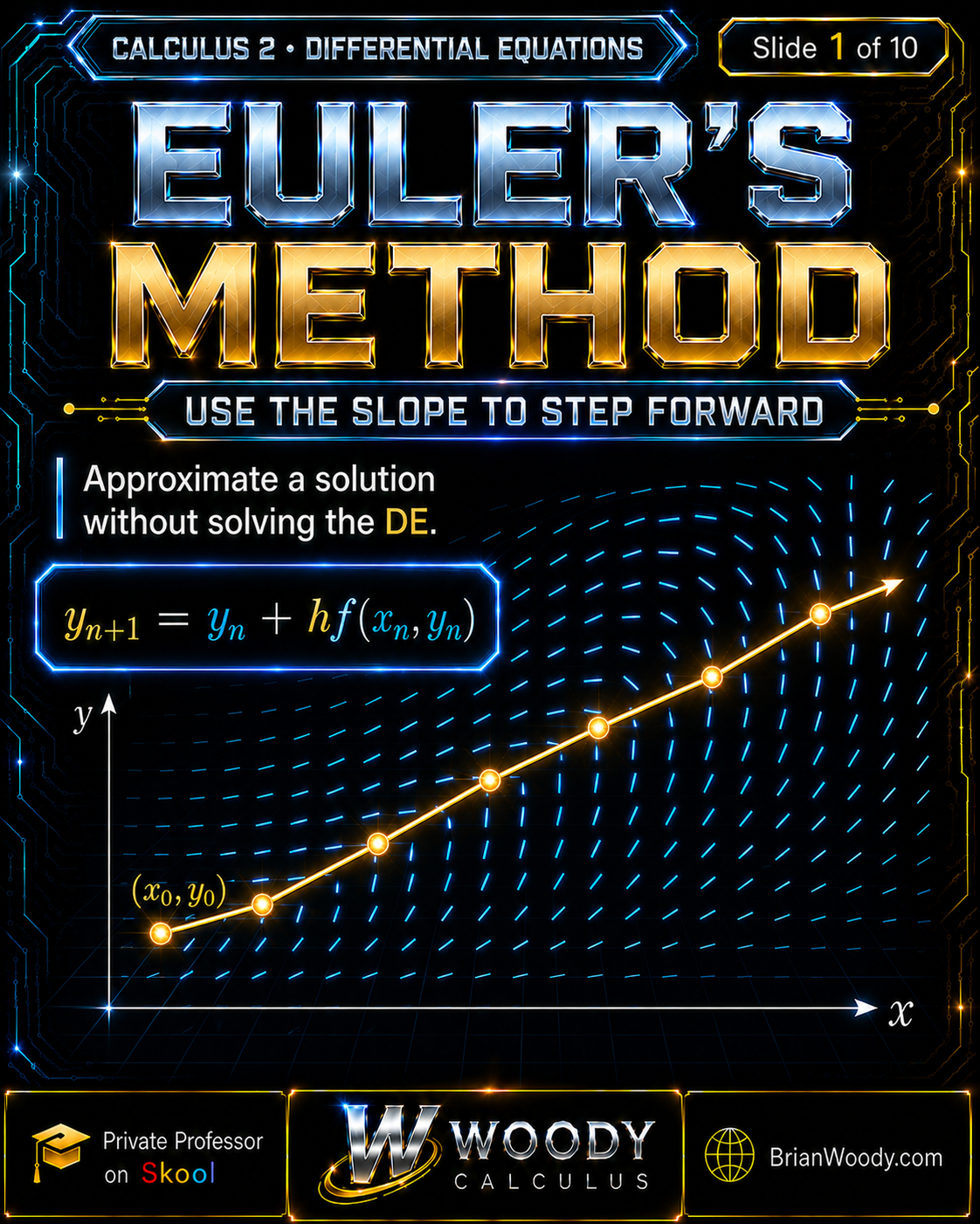
Euler’s method approximates the solution of an initial-value problem by repeatedly using the differential equation’s slope. Learn the update formula, complete a worked example, compare step sizes, and verify the approximation against an exact solution.

How do you decide whether to use separation of variables or an integrating factor? This Woody Calculus lesson explains how to classify separable and first-order linear differential equations, solve each type step by step, handle equations that fit both methods, and verify the final solution.