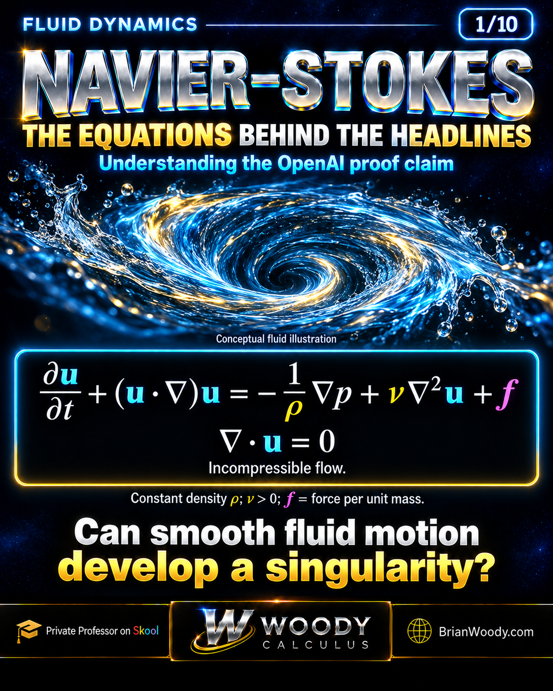

What does Navier–Stokes actually say—and what does the OpenAI announcement claim? Decode every term, verify exact fluid solutions, calculate energy decay, and test your understanding with 12 worked practice problems.
What does Navier–Stokes actually say—and what does the OpenAI announcement claim? Decode every term, verify exact fluid solutions, calculate energy decay, and test your understanding with 12 worked practice problems.
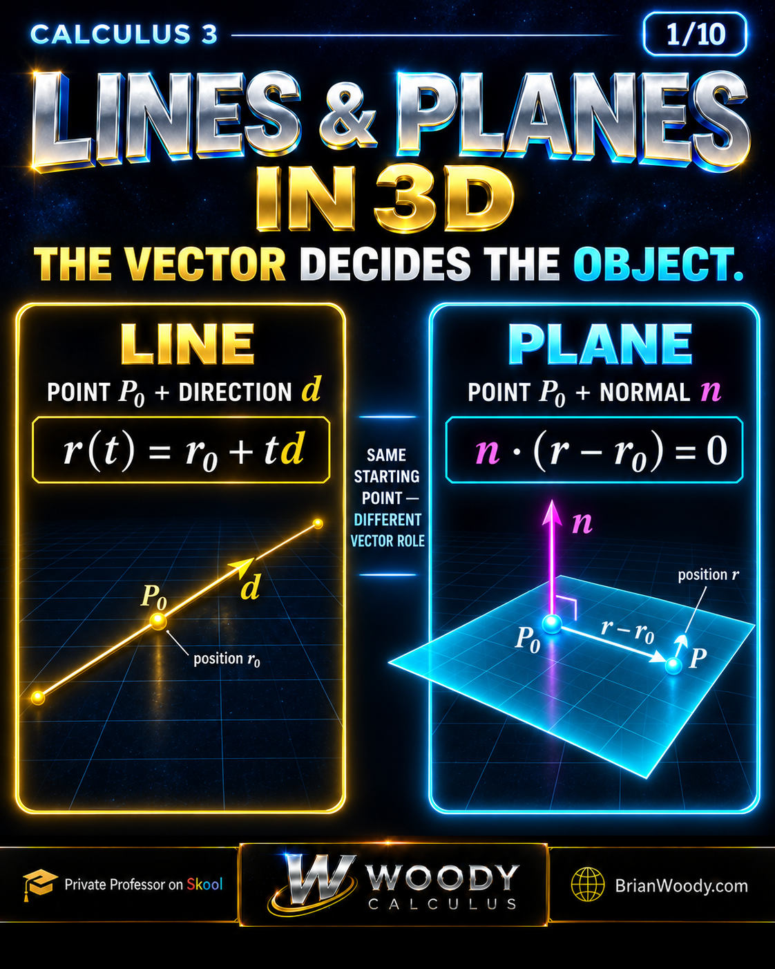
Learn how points, direction vectors, and normal vectors build lines and planes in three dimensions. Work through equations, intersections, distances, and tangent-plane normals with 10 visual slides and 12 practice problems with solutions.
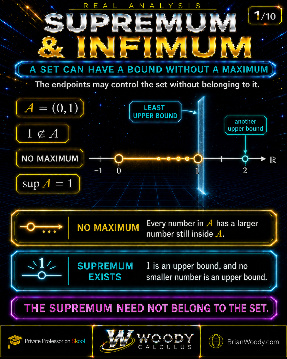
Learn how upper and lower bounds lead to supremum, infimum, maximum, and minimum. This complete Real Analysis lesson includes epsilon proofs, sequence examples, the completeness axiom, and a rigorous explanation of why the rational numbers have gaps.
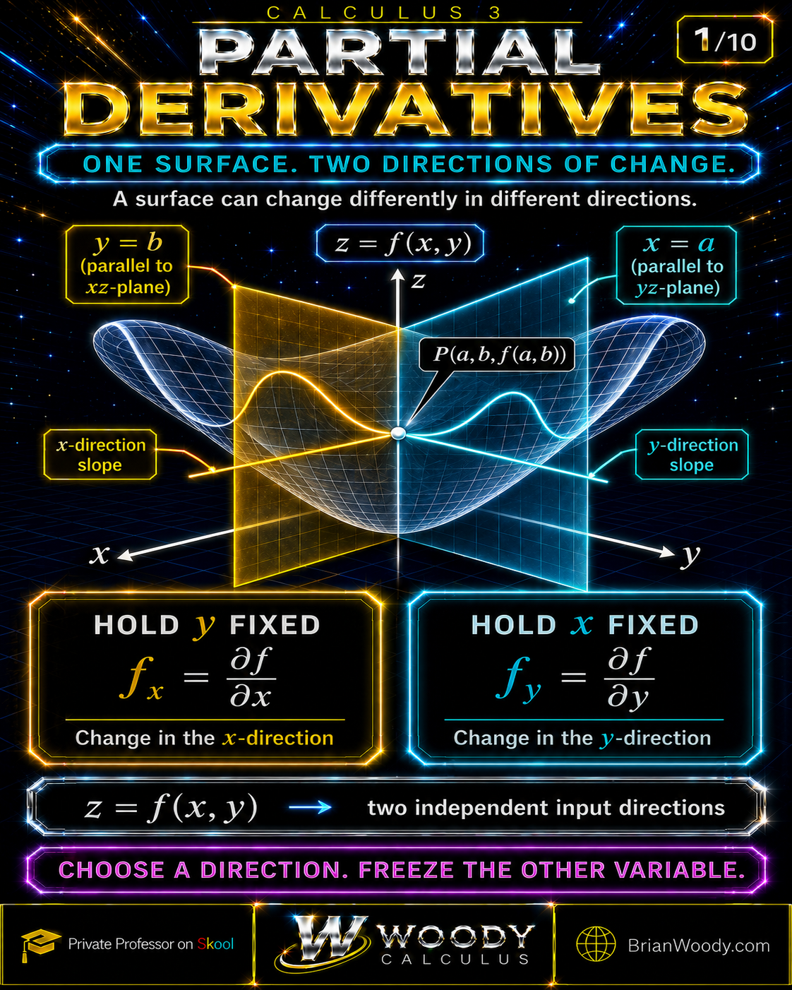
Partial derivatives measure how a multivariable function changes when one input varies and the others are held constant. This complete Calculus 3 lesson develops limit definitions, trace curves, first and mixed partials, tangent planes, the multivariable chain rule, linear approximation, rigorous counterexamples, and solved practice problems.
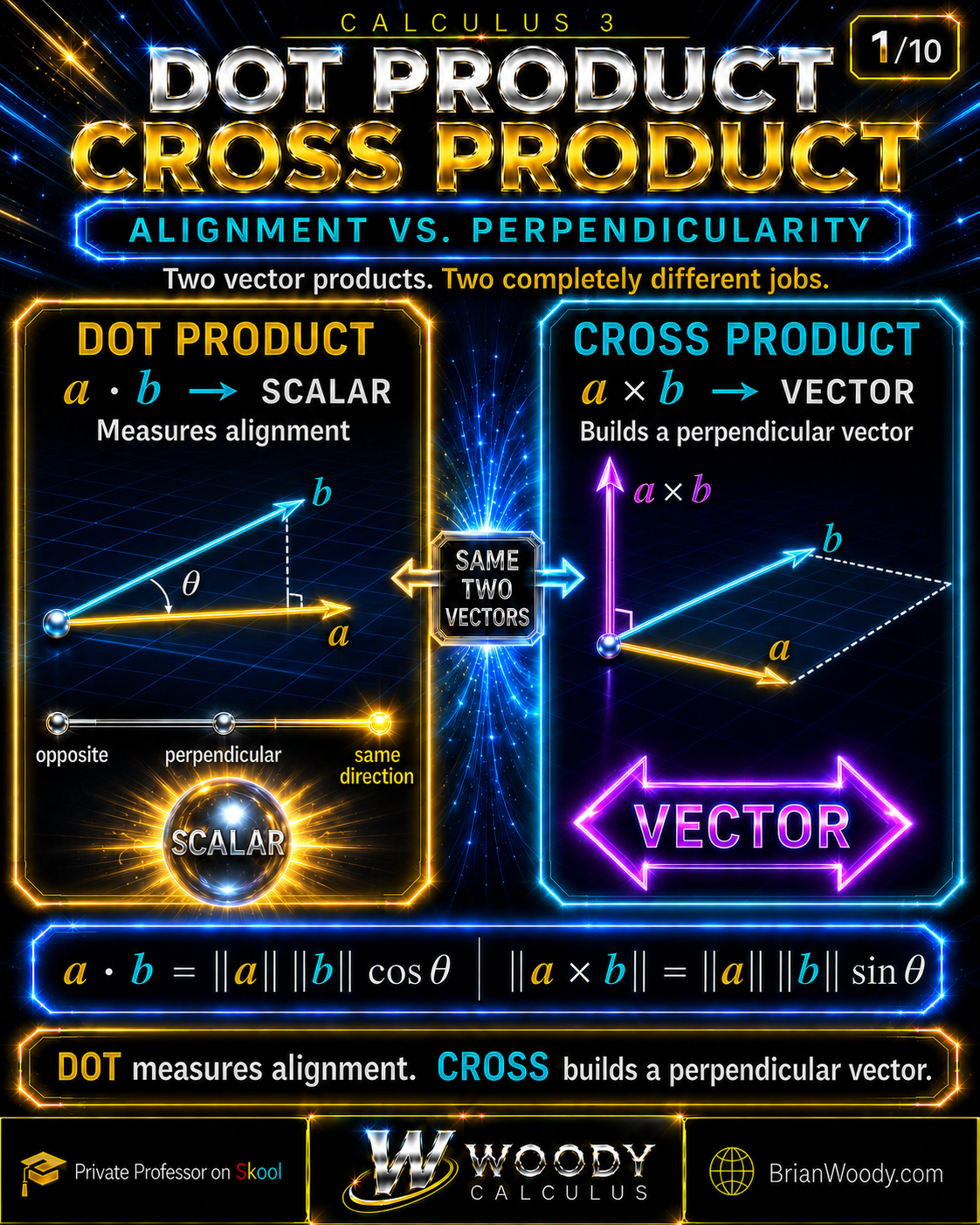
The dot product returns a scalar that measures alignment, while the cross product returns a vector perpendicular to two three-dimensional vectors. Learn the formulas, geometric meaning, right-hand rule, projections, work, area, plane normals, torque, flux, scalar triple products, Lagrange’s identity, and complete worked examples.
![Woody Calculus introduction to differential-equation mixing problems, showing a perfectly stirred saltwater tank with inflow and outflow. The governing model is Q′(t) = c_in r_in − [Q(t)/V(t)]r_out. Equal flow rates produce constant volume, while unequal flow rates produce changing volume.](https://k3p6r8v3.delivery.rocketcdn.me/wp-content/uploads/2026/08/Mixing_Problems_Slide_01.png)
Learn how to model and solve differential-equation mixing problems with rate in minus rate out. Work through constant-volume, draining-tank, and overflow examples, then practice the complete seven-step method.
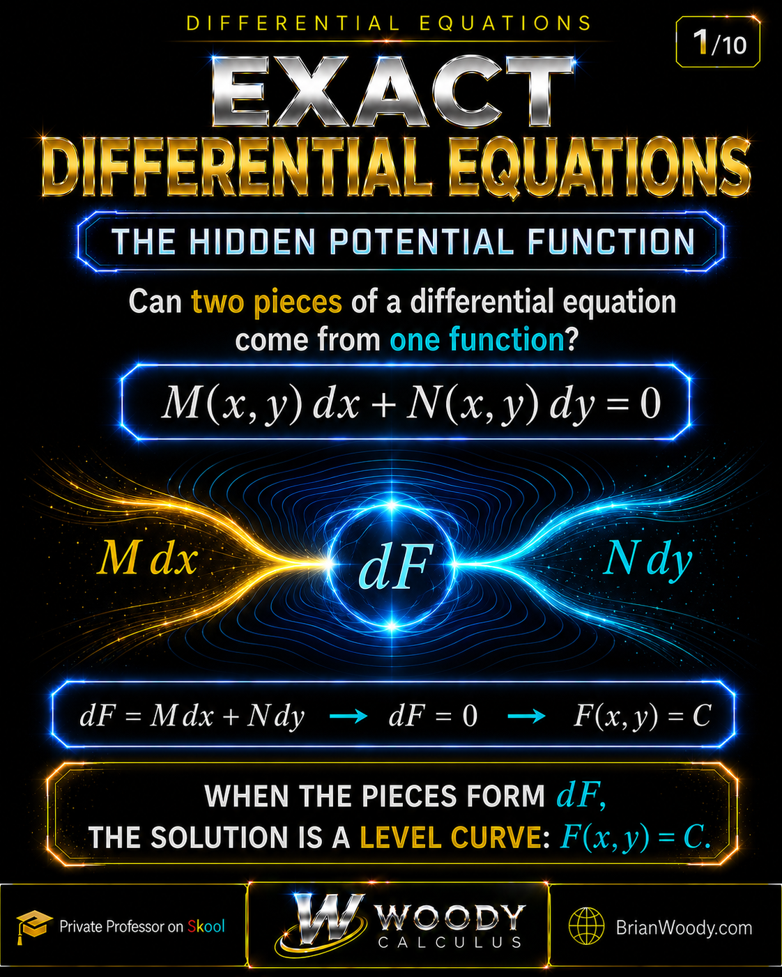
Learn how to recognize and solve exact differential equations using the exactness test M_y = N_x, recover a potential function F(x,y), apply initial conditions, verify implicit solutions, and use special integrating factors when an equation is not exact. This rigorous visual lesson also explains domain restrictions, conservative vector fields, line integrals, and the punctured-domain caveat.
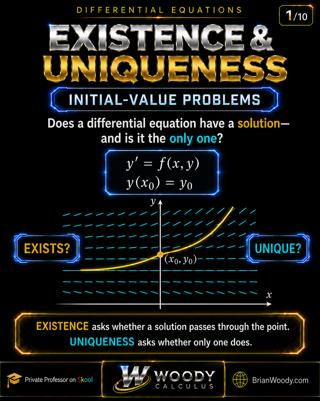
Does an initial-value problem have a solution, and is that solution the only one? This complete Woody Calculus lesson explains the existence and uniqueness theorem, the rectangle test, worked examples, nonunique solutions, finite-time blow-up, maximal intervals, the nonintersection principle, and higher-order linear ODEs.
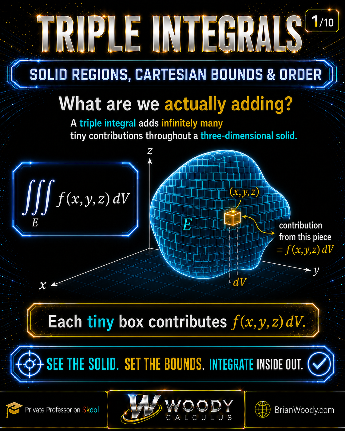
Triple integrals become manageable when you see the solid first. Learn how to choose a projection, write valid Cartesian bounds, integrate inside out, change the order of integration, and calculate volume, mass, average value, and center of mass through exact worked examples.
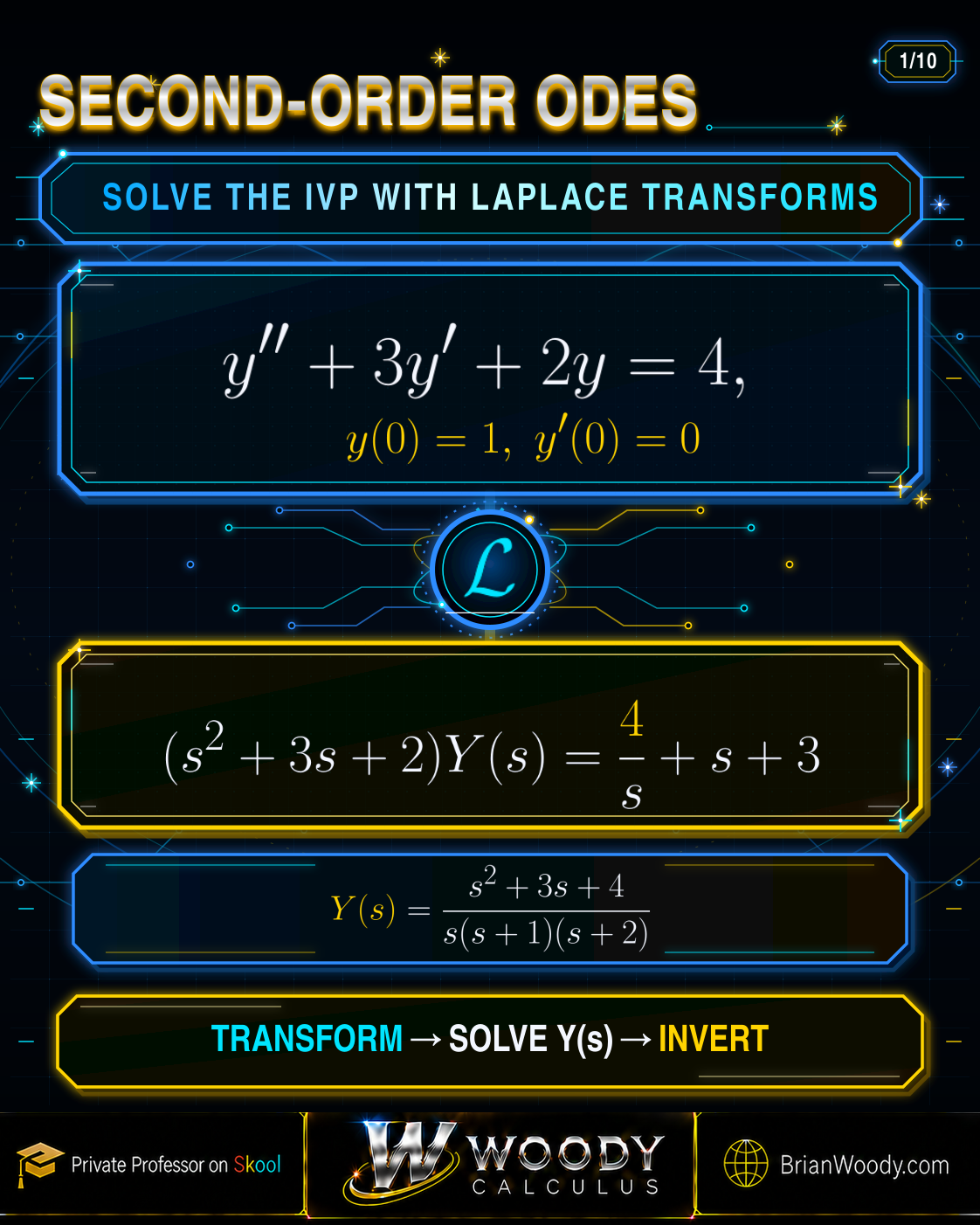
Laplace transforms turn second-order initial-value problems into algebra while carrying the initial conditions with them. Learn the complete seven-step method, partial fractions, delayed unit-step inputs, Dirac delta impulses, transfer functions, impulse response, convolution, stability, and verification through exact worked examples.