A power series solution of a differential equation represents the unknown function as
\(y=\sum_{n=0}^{\infty}a_nx^n\) and uses the Five-Stage Power Series Method: Assume, Differentiate, Substitute, Reindex, and Recur. For the Airy equation \(y^{\prime\prime}-xy=0\), the method produces
\(a_2=0\) and
\(a_{n+2}=\frac{a_{n-1}}{(n+2)(n+1)}\) for \(n\ge1\), with \(a_0=y(0)\) and \(a_1=y^{\prime}(0)\) as the two free constants.
Plain-language answer:
the Five-Stage Power Series Method turns an unknown function into an organized coefficient sequence: assume the series, differentiate it, substitute it, align its powers, and derive the recurrence.
What should you know before solving an ODE with a power series?
You should know power series notation, term-by-term differentiation, index shifting, and the basic classification of differential equations.
- How to write \(\sum_{n=0}^{\infty}a_nx^n\) as \(a_0+a_1x+a_2x^2+\cdots\)
- How to differentiate powers of \(x\)
- How to reindex a series without changing its terms
- How to recognize a linear second-order ODE and identify an ordinary point
- Why equal power series have equal coefficients
Quick Summary: Power Series Solutions of Differential Equations
The Five-Stage Power Series Method is: Assume, Differentiate, Substitute, Reindex, and Recur. After the powers are aligned, equate coefficients and use the recurrence relation to build the solution.
- Classify the ODE and verify that the expansion point is ordinary.
- Write \(y\), \(y^{\prime}\), and \(y^{\prime\prime}\) with aligned powers.
- Substitute every series into the original differential equation.
- Separate any low-degree terms that do not fit the common index range.
- Set each coefficient equal to zero and solve the recurrence.
- Use the initial conditions to determine the free coefficients.
Key Facts
- Five-Stage Power Series Method: Assume → Differentiate → Substitute → Reindex → Recur.
- Airy equation: \(y^{\prime\prime}-xy=0\).
- Expansion point: \(x=0\), which is an ordinary point.
- Recurrence: \(a_{n+2}=\frac{a_{n-1}}{(n+2)(n+1)}\) for \(n\ge1\).
- Free data: \(a_0=y(0)\) and \(a_1=y^{\prime}(0)\).
- Coefficient pattern: the indices split into three chains modulo 3, and the \(a_{3k+2}\) chain is zero.
- Convergence: both nonzero basis series converge for every real or complex \(x\).
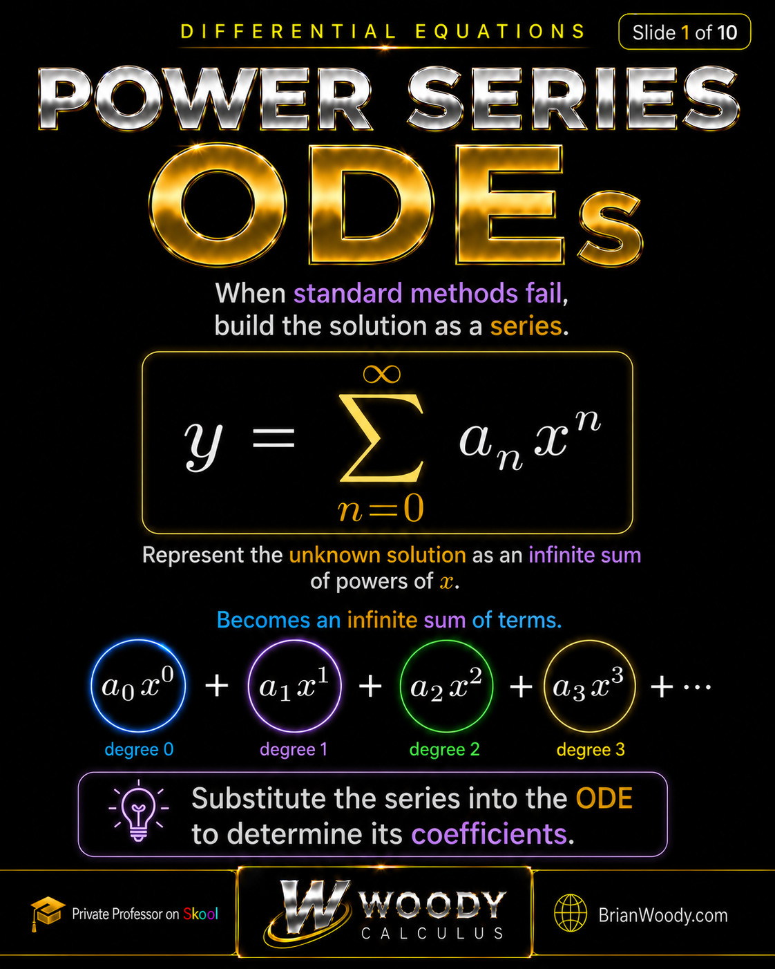
What is the power series method for differential equations?
The power series method replaces an unknown function with an infinite polynomial whose coefficients are determined by the differential equation.
Around the expansion point \(x=0\), assume
y=\sum_{n=0}^{\infty}a_nx^n
=a_0+a_1x+a_2x^2+a_3x^3+\cdots.
\]
The coefficients \(a_0,a_1,a_2,\ldots\) are initially unknown. The ODE creates algebraic relationships among them. Once those relationships are found, the function is built coefficient by coefficient.
Plain-language answer:
the differential equation becomes a machine that generates the Taylor coefficients of its solution.
What does the power series notation mean?
The index \(n\) labels the power of \(x\), while \(a_n\) is the coefficient attached to that power.
| Symbol | Meaning | Role in the method |
|---|---|---|
| \(a_n\) | The coefficient of \(x^n\) | The recurrence relation determines these values. |
| \(n\) | A nonnegative integer index | It labels the degree of each term. |
| \(a_0\) | The constant coefficient | For expansion at 0, \(a_0=y(0)\). |
| \(a_1\) | The coefficient of \(x\) | For expansion at 0, \(a_1=y^{\prime}(0)\). |
| Recurrence relation | A formula connecting later coefficients to earlier ones | It replaces the differential equation with an algebraic rule. |
| Ordinary point | A point where the normalized coefficient functions are analytic | An ordinary power series may be used around that point. |
When should you use a power series to solve an ODE?
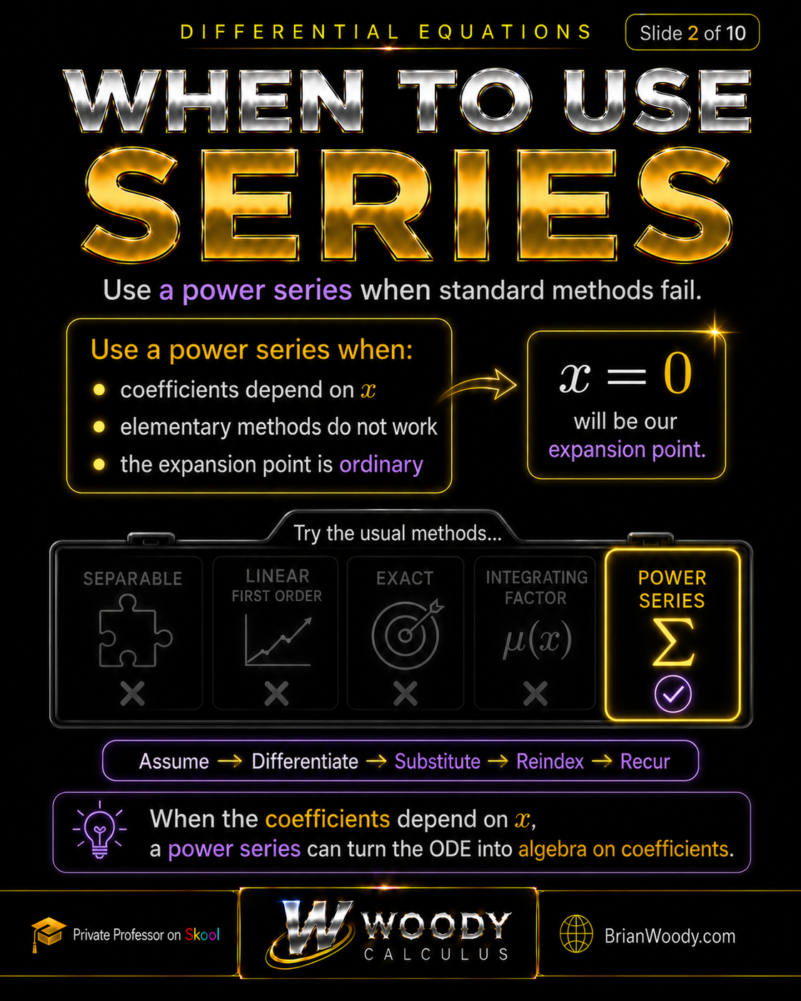
Use the power series method when the ODE has analytic coefficients near an ordinary point and a local analytic solution is desired, especially when standard elementary methods do not produce a useful closed form.
Variable coefficients alone do not automatically force a power series method. Classification still comes first. A variable-coefficient equation may be separable, first-order linear, exact, reducible, or otherwise solvable. The power series method becomes especially valuable after those simpler structures have been ruled out or when the series itself is the desired form.
| Structure near the point | Method to consider | Recognition clue |
|---|---|---|
| Elementary first-order structure | Separable, linear, exact, or integrating factor | The equation matches a standard first-order form. |
| Constant-coefficient linear ODE | Characteristic equation | The coefficients of \(y,y^{\prime},y^{\prime\prime}\) are constants. |
| Ordinary point with analytic coefficients | Ordinary power series | The normalized coefficient functions are analytic at the expansion point. |
| Regular singular point | Frobenius method | An ordinary power series may fail, but the singularity is controlled after multiplication by appropriate powers of \(x-x_0\). |
| Initial-value problem with forcing or discontinuities | Laplace transforms | Piecewise inputs, impulses, or transform-friendly data are present. |
For transform-based initial-value problems, compare this method with
Laplace transforms for differential equations.
For numerical approximation rather than an exact analytic series, review
Euler’s Method.
What is an ordinary point in a differential equation?
For \(A(x)y^{\prime\prime}+B(x)y^{\prime}+C(x)y=0\), a point \(x_0\) is ordinary when \(A(x_0)\ne0\) and the normalized functions \(B/A\) and \(C/A\) are analytic near \(x_0\).
Ordinary-Point Test
Normalize the equation to
y^{\prime\prime}+P(x)y^{\prime}+Q(x)y=0.
\]
If \(P\) and \(Q\) are analytic near \(x_0\), then \(x_0\) is an ordinary point and the local solution can be represented by a convergent power series centered at \(x_0\).
For the Airy equation
y^{\prime\prime}-xy=0,
\]
we have \(P(x)=0\) and \(Q(x)=-x\). Both are polynomials, so every finite point is ordinary. In particular, \(x=0\) is an ideal expansion point.
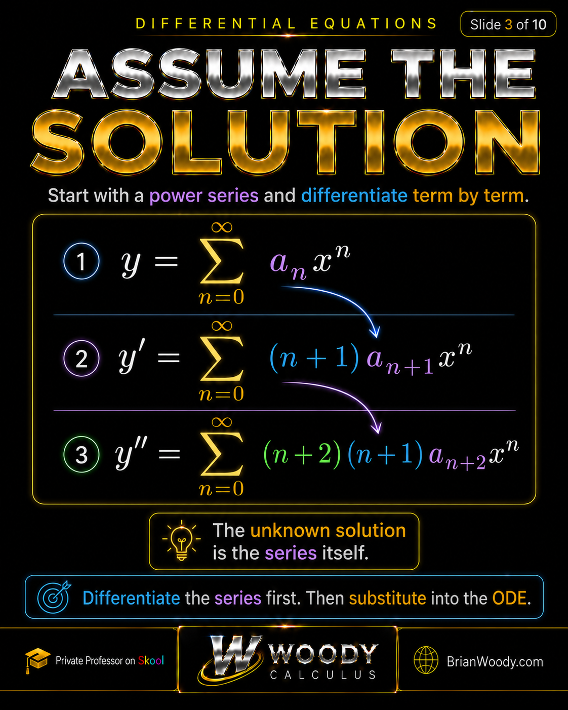
How do you differentiate the assumed power series?
Differentiate term by term and then reindex the derivatives so that each series is written in powers of \(x^n\).
y=\sum_{n=0}^{\infty}a_nx^n.
\]
y^{\prime}
=\sum_{n=1}^{\infty}na_nx^{n-1}
=\sum_{n=0}^{\infty}(n+1)a_{n+1}x^n.
\]
y^{\prime\prime}
=\sum_{n=2}^{\infty}n(n-1)a_nx^{n-2}
=\sum_{n=0}^{\infty}(n+2)(n+1)a_{n+2}x^n.
\]
Why is the Airy equation a good power series example?
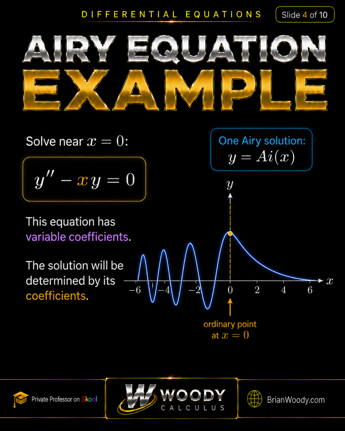
The Airy equation is linear, has a variable coefficient, is ordinary at \(x=0\), and does not yield to the constant-coefficient characteristic-equation method.
y^{\prime\prime}-xy=0.
\]
The equation is second order, so its general solution must contain two independent constants. A traditional named basis is \(\operatorname{Ai}(x)\) and \(\operatorname{Bi}(x)\), but the power series method constructs an equally valid basis directly from the initial coefficients \(a_0\) and \(a_1\).
The graph of \(\operatorname{Ai}(x)\) is oscillatory for negative \(x\) and decays for positive \(x\). The slide gives a qualitative schematic of that behavior.
How do you substitute the power series into the Airy equation?
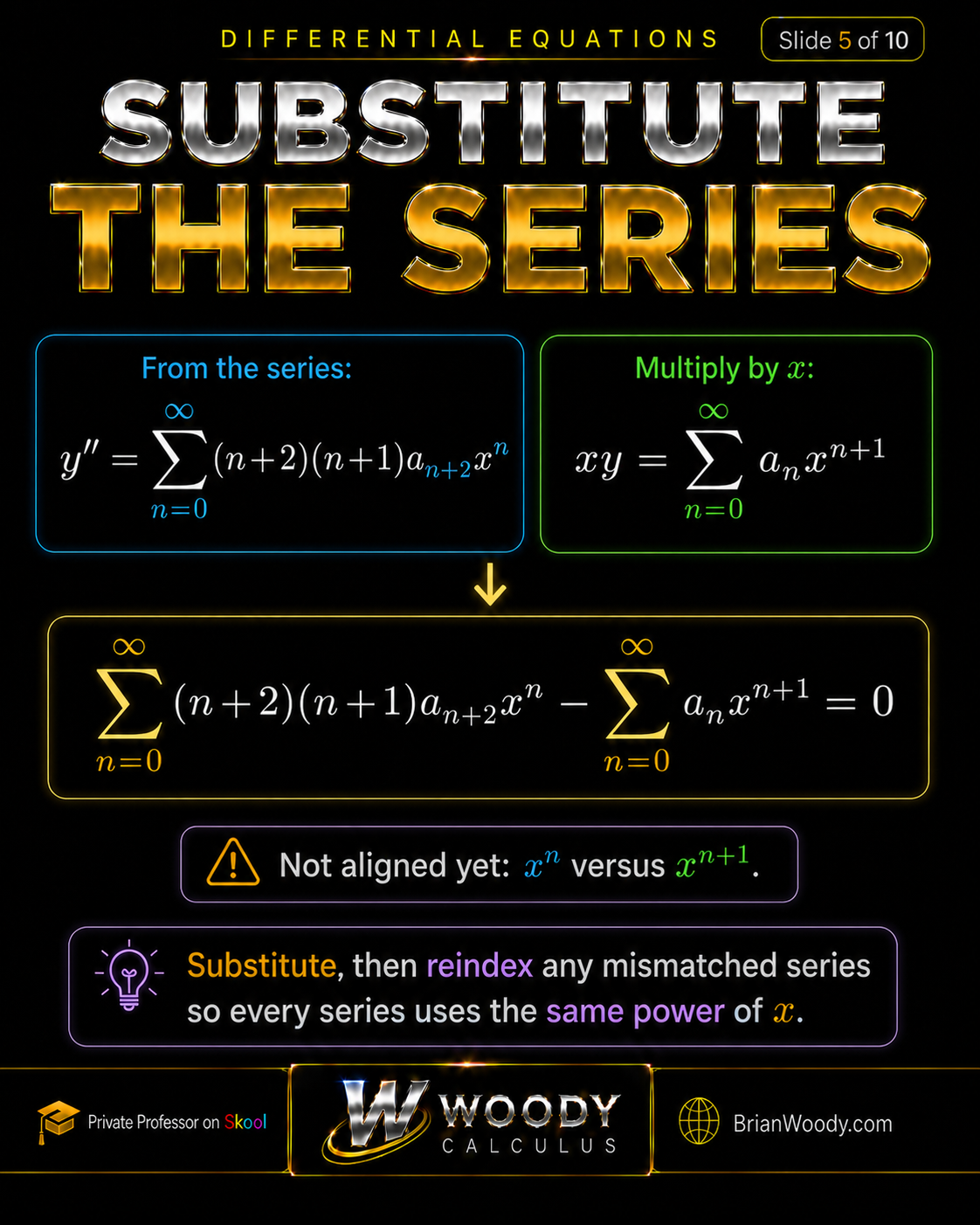
Replace \(y^{\prime\prime}\) by its differentiated series and replace \(xy\) by the original series multiplied by \(x\).
y^{\prime\prime}
=\sum_{n=0}^{\infty}(n+2)(n+1)a_{n+2}x^n.
\]
xy
=x\sum_{n=0}^{\infty}a_nx^n
=\sum_{n=0}^{\infty}a_nx^{n+1}.
\]
Substituting into \(y^{\prime\prime}-xy=0\) gives
\sum_{n=0}^{\infty}(n+2)(n+1)a_{n+2}x^n
-\sum_{n=0}^{\infty}a_nx^{n+1}
=0.
\]
Plain-language answer:
substitution is not the difficult step; the real work is making both sums speak the same power-of-\(x\) language.
How do you reindex the series so the powers match?
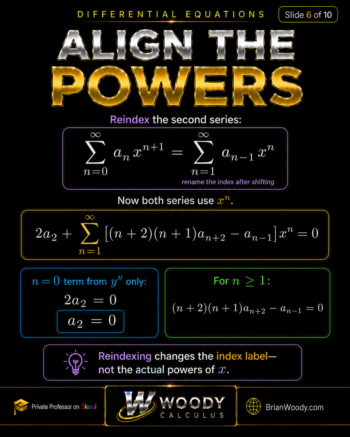
Rewrite the second sum in powers of \(x^n\) by shifting its index from \(n=0\) to \(n=1\).
\sum_{n=0}^{\infty}a_nx^{n+1}
=\sum_{n=1}^{\infty}a_{n-1}x^n.
\]
The first series begins at \(n=0\), while the reindexed second series begins at \(n=1\). Therefore, separate the \(n=0\) term of the first series:
2a_2
+\sum_{n=1}^{\infty}
\left[(n+2)(n+1)a_{n+2}-a_{n-1}\right]x^n
=0.
\]
Reindexing rule
Reindexing changes the label attached to each term, not the terms themselves. Always check the first term before and after the shift.
How do you derive the recurrence relation?
A power series is identically zero only when every coefficient is zero, so the constant term and every coefficient of \(x^n\) must vanish separately.
From the constant term,
2a_2=0
\quad\Longrightarrow\quad
\boxed{a_2=0}.
\]
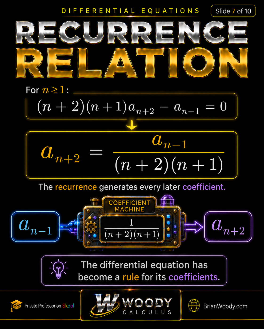
For every \(n\ge1\),
(n+2)(n+1)a_{n+2}-a_{n-1}=0.
\]
Solving for the later coefficient gives the recurrence relation
\boxed{
a_{n+2}=\frac{a_{n-1}}{(n+2)(n+1)},
\qquad n\ge1.
}
\]
Plain-language answer:
every coefficient three places later is generated from an earlier coefficient by dividing by two consecutive integers.
How do you build the power series coefficients?
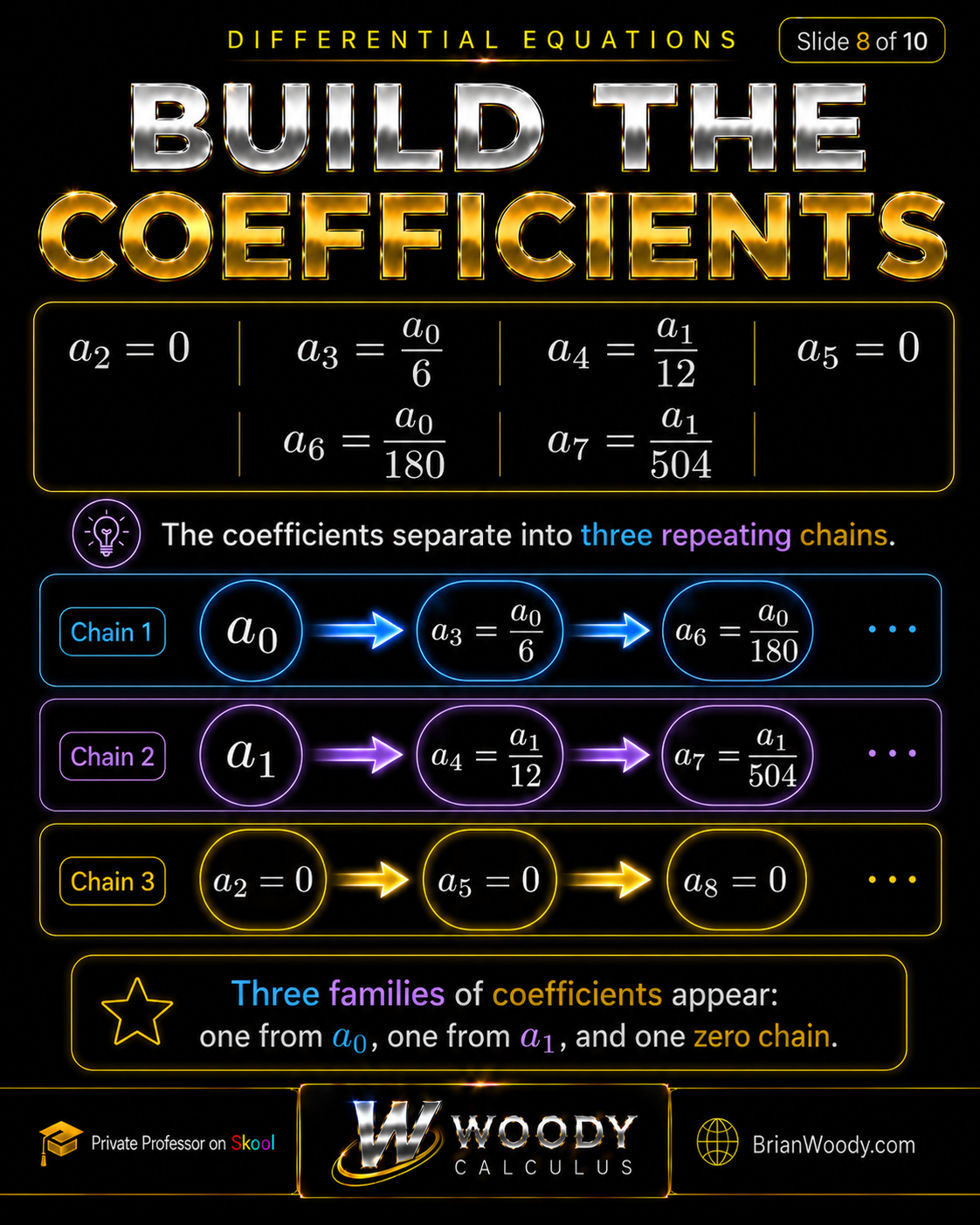
Insert \(n=1,2,3,\ldots\) into the recurrence and track the three index classes modulo 3.
| Index choice | Coefficient | Result |
|---|---|---|
| Constant term | \(2a_2=0\) | \(a_2=0\) |
| \(n=1\) | \(a_3=\frac{a_0}{3\cdot2}\) | \(a_3=\frac{a_0}{6}\) |
| \(n=2\) | \(a_4=\frac{a_1}{4\cdot3}\) | \(a_4=\frac{a_1}{12}\) |
| \(n=3\) | \(a_5=\frac{a_2}{5\cdot4}\) | \(a_5=0\) |
| \(n=4\) | \(a_6=\frac{a_3}{6\cdot5}\) | \(a_6=\frac{a_0}{180}\) |
| \(n=5\) | \(a_7=\frac{a_4}{7\cdot6}\) | \(a_7=\frac{a_1}{504}\) |
| \(n=6\) | \(a_8=\frac{a_5}{8\cdot7}\) | \(a_8=0\) |
The recurrence jumps by three indices, so the coefficients split into three independent chains:
a_0\to a_3\to a_6\to a_9\to\cdots,
\]
a_1\to a_4\to a_7\to a_{10}\to\cdots,
\]
a_2=0\to a_5=0\to a_8=0\to\cdots.
\]
Why do the \(x^2\), \(x^5\), and \(x^8\) terms vanish?
They vanish because the constant-term equation forces \(a_2=0\), and the recurrence then carries that zero forward through every index congruent to 2 modulo 3.
The recurrence links coefficients three indices apart. Once \(a_2=0\), it follows that
\(a_5=\frac{a_2}{5\cdot4}=0\), then
\(a_8=\frac{a_5}{8\cdot7}=0\), and so on. Therefore the exact Airy series contains no terms of degree \(3k+2\).
What is the general power series solution of the Airy equation?
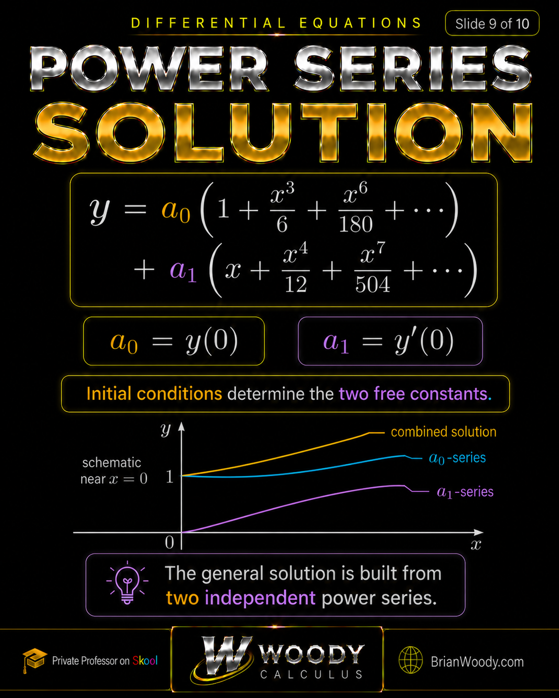
The general solution is a linear combination of one series generated by \(a_0\) and a second independent series generated by \(a_1\).
\begin{aligned}
y(x)
={}&a_0\left(
1+\frac{x^3}{6}+\frac{x^6}{180}+\frac{x^9}{12960}+\cdots
\right)\\
&+a_1\left(
x+\frac{x^4}{12}+\frac{x^7}{504}+\frac{x^{10}}{45360}+\cdots
\right).
\end{aligned}
\]
The two series are linearly independent because the first has initial data \(y(0)=1\), \(y^{\prime}(0)=0\), while the second has initial data \(y(0)=0\), \(y^{\prime}(0)=1\). Their Wronskian at \(x=0\) is therefore 1.
What do the free coefficients mean?
Since this is a second-order linear homogeneous ODE, two independent constants are required. In the power series basis, those constants are exactly
\(a_0=y(0)\) and \(a_1=y^{\prime}(0)\).
How do initial conditions determine a power series solution?
At an expansion point of 0, the initial conditions directly set \(a_0=y(0)\) and \(a_1=y^{\prime}(0)\).
How can you independently verify the power series solution?
Differentiate the truncated series, substitute it back into the ODE, check the initial data, and verify the convergence of both coefficient chains.
How does the power series solution connect to Airy functions?
The two power series built from \(a_0\) and \(a_1\) form a fundamental solution set, so the named Airy functions \(\operatorname{Ai}(x)\) and \(\operatorname{Bi}(x)\) are fixed linear combinations of them.
y=C_1\operatorname{Ai}(x)+C_2\operatorname{Bi}(x).
\]
The power series basis and the Airy-function basis describe the same two-dimensional solution space. The advantage of the power series basis is that its constants have the immediate interpretation \(a_0=y(0)\) and \(a_1=y^{\prime}(0)\).
For an authoritative reference on the differential equation, graphs, and Maclaurin series of Airy functions, see the
NIST Digital Library of Mathematical Functions, Chapter 9.
Advanced insight: the nearest-singularity rule
For a linear ODE with analytic normalized coefficients, the power series centered at an ordinary point converges at least as far as the nearest singularity of those coefficients. In the Airy equation, the normalized coefficients are polynomials and have no finite singularities, which agrees with the infinite radius obtained directly from the recurrence.
What mistakes do students make with power series solutions of ODEs?
Most errors come from choosing the method before classifying the equation, differentiating with the wrong index, reindexing incorrectly, or equating coefficients before the powers match.
Mistake: Using a power series before classifying the ODE
Symptom: A long series calculation begins even though the equation is separable, first-order linear, or constant coefficient.
Cause: The method was selected from appearance instead of structure.
Fix: Classify first. Use power series after checking for simpler exact methods or when the series form is specifically requested.
Mistake: Confusing an ordinary point with a regular singular point
Symptom: The student uses an ordinary series where the leading coefficient vanishes at the expansion point.
Cause: The equation was not normalized before testing the coefficients.
Fix: Divide by the leading coefficient first. If the point is regular singular rather than ordinary, consider the Frobenius method.
Mistake: Differentiating the coefficient instead of the power
Symptom: The derivative is written as \(\sum a_nx^{n-1}\) with the factor \(n\) missing.
Cause: The power rule was applied incompletely.
Fix: Differentiate one generic term: \(\frac{d}{dx}(a_nx^n)=na_nx^{n-1}\).
Mistake: Reindexing only the exponent
Symptom: \(\sum a_nx^{n+1}\) is changed to \(\sum a_nx^n\) without changing the coefficient or lower limit.
Cause: The index label was changed inconsistently.
Fix: Verify the first term before and after reindexing. Here, \(\sum_{n=0}^{\infty}a_nx^{n+1}=\sum_{n=1}^{\infty}a_{n-1}x^n\).
Mistake: Forgetting the unmatched \(n=0\) term
Symptom: The student writes one combined sum beginning at \(n=1\) and loses the equation \(2a_2=0\).
Cause: The lower limits were aligned without separating the extra term.
Fix: Isolate every term below the common starting index before combining sums.
Mistake: Using the recurrence at an invalid index
Symptom: The formula for \(a_{n+2}\) is applied at \(n=0\), producing an undefined \(a_{-1}\).
Cause: The condition \(n\ge1\) was ignored.
Fix: Handle the constant term separately, then apply the recurrence only for \(n\ge1\).
Mistake: Expecting one free constant in a second-order equation
Symptom: The final solution contains only the \(a_0\)-series or only the \(a_1\)-series.
Cause: The order of the differential equation was not connected to the dimension of the solution space.
Fix: Preserve both free coefficients unless two initial conditions determine them.
Mistake: Treating a truncated series as the exact entire solution
Symptom: The student writes a polynomial approximation with no ellipsis and calls it the complete solution.
Cause: Approximation and equality were confused.
Fix: Keep the infinite-series notation for the exact solution and label finite truncations as approximations.
Woody Calculus rule
Do not reindex mentally. Write the old index, the substitution, the new lower limit, and the renamed index. Most power series errors are organization errors before they are calculus errors.
What is the Woody Calculus exam checklist for power series ODEs?
Classify first. Assume second. Align third. Recur fourth. Verify last.
- Write the ODE in standard form.
- Identify the expansion point and verify that it is ordinary.
- State the assumed power series from memory.
- Differentiate term by term and align the derivative powers.
- Substitute every series into the original ODE.
- Reindex until all sums use the same power of \(x\).
- Separate any low-degree terms outside the common range.
- Set each coefficient equal to zero.
- State the recurrence relation with its correct index range.
- Generate enough coefficients to reveal the pattern.
- Preserve the correct number of free constants.
- Apply initial conditions only after identifying \(a_0\) and \(a_1\).
- Substitute the first terms back into the ODE as a verification.
- Rebuild the complete solution from a blank page and say every index shift aloud.
Formula memorization is required, but the equation’s structure chooses the formula. Memorize the derivative shifts and the workflow; then let the ODE determine the recurrence.
How do you master power series solutions of differential equations?
Mastery means you can move from an analytic ODE to a recurrence relation without losing an index, a low-degree term, or a free constant.
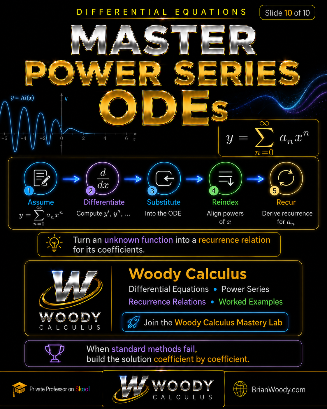
The Five-Stage Power Series Method
- Assume: write \(y=\sum a_nx^n\).
- Differentiate: compute and align \(y^{\prime},y^{\prime\prime},\ldots\).
- Substitute: place every series into the ODE.
- Reindex: express every sum using the same power.
- Recur: equate coefficients and generate the solution.
Reading a recurrence is not enough. Re-derive it. Rewrite the perfect solution until the index shifts become automatic, then solve a nearby problem with a different coefficient or expansion point.
Frequently Asked Questions About Power Series Solutions of ODEs
What is a power series solution of a differential equation?
A power series solution represents the unknown function as an infinite sum \(y=\sum_{n=0}^{\infty}a_nx^n\). Substitution into the differential equation produces algebraic equations or a recurrence relation for the coefficients.
When should you use the power series method?
Use the power series method near an ordinary point when the normalized coefficient functions are analytic and standard elementary methods do not give a useful solution, or when a local series representation is specifically required.
What is an ordinary point?
For a normalized second-order equation \(y^{\prime\prime}+P(x)y^{\prime}+Q(x)y=0\), an ordinary point is a point where \(P\) and \(Q\) are analytic. An ordinary power series may be centered there.
Why must the powers of x be aligned before equating coefficients?
Coefficients can be compared only when they multiply the same power of \(x\). Reindexing rewrites each series in a common form without changing its terms.
What is the recurrence relation for the Airy equation?
For \(y^{\prime\prime}-xy=0\), the constant term gives \(a_2=0\), and the remaining coefficients satisfy \(a_{n+2}=a_{n-1}/((n+2)(n+1))\) for \(n\ge1\).
Why do the Airy coefficients split into three chains?
The recurrence connects \(a_{n+2}\) to \(a_{n-1}\), which changes the index by three. Therefore the coefficients separate according to their indices modulo 3.
How do initial conditions enter the power series solution?
For a series centered at 0, \(a_0=y(0)\) and \(a_1=y^{\prime}(0)\). These two values determine the two free constants in the general solution of the second-order equation.
How is the power series solution related to Ai and Bi?
The two series generated by \(a_0\) and \(a_1\) form a fundamental solution set for the Airy equation. The named functions \(\operatorname{Ai}(x)\) and \(\operatorname{Bi}(x)\) are fixed linear combinations of that series basis.
Does the Airy power series converge for every x?
Yes. The ratio of successive terms in each nonzero coefficient chain tends to zero for every fixed \(x\), so both basis series have infinite radius of convergence.
How do you solve \(y^{\prime\prime}-xy=0\) with a power series?
Assume \(y=\sum_{n=0}^{\infty}a_nx^n\), differentiate twice, substitute into the equation, and reindex the \(xy\) series. The constant term gives \(a_2=0\), while the remaining coefficients satisfy \(a_{n+2}=a_{n-1}/((n+2)(n+1))\) for \(n\ge1\).
Why are there no \(x^2\), \(x^5\), or \(x^8\) terms in the Airy series?
The constant-term equation forces \(a_2=0\). Because the recurrence advances that coefficient chain by three indices, it then forces \(a_5=a_8=a_{11}=\cdots=0\).
What is the difference between the power series method and the Frobenius method?
The ordinary power series method assumes integer powers beginning with \(x^0\) and is used at an ordinary point. The Frobenius method assumes \(y=\sum_{n=0}^{\infty}a_n(x-x_0)^{n+r}\) and is designed for regular singular points, where the exponent \(r\) is determined by an indicial equation.
Need help with university differential equations?
The
Woody Calculus Mastery Lab
is the required starting point for students who want help with differential equations, power series, Laplace transforms, systems, and exam preparation.
Limited
private instruction
may be available after Mastery Lab enrollment. It is selective, limited, normally based on weekly sessions, and not guaranteed.
Visit the
contact page
or explore the
university mathematics help hub.
University differential equations help
Purdue differential equations support
Professor-led help with power series, Laplace transforms, systems, and exam preparation.
University of Florida mathematics support
Structured help for students working through university differential equations and advanced calculus.
UCF differential equations help
Support with method selection, complete solutions, recurrence relations, and final-exam preparation.
Auburn mathematics support
Strengthen differential equations technique, notation, and independent problem solving.
University of Alabama mathematics support
Build a reliable workflow for ODE classification, solution methods, and verification.
UNR differential equations support
University-level help from a former lecturer with deep experience teaching differential equations.
Reviews and trust
Read
Woody Calculus 5-star Google reviews
and view
Brian M. Woody’s 5.0 RateMyProfessors rating.
Woody Calculus provides university-level mathematical instruction, structured practice, and long-term mastery—not generic tutoring and not a shortcut answer service.