Phase portraits are one of the most powerful visual tools in Differential Equations. They let you look at a linear system and predict the future from the eigenvalues.
For a two-dimensional linear system,
\vec{x}^{\prime}=A\vec{x},
\]
the eigenvalues of the matrix \(A\) tell you whether solutions move toward the origin, away from the origin, spiral inward, spiral outward, orbit around the origin, or split into stable and unstable directions. That is why phase portraits connect eigenvalues and eigenvectors directly to geometric motion.
For a 2×2 linear system, phase portraits let you predict stability by analyzing the coefficient matrix. By solving the characteristic equation
\det(A-\lambda I)=0,
\]
you classify the equilibrium as a node, saddle point, spiral, center, or repeated-eigenvalue case and predict whether nearby solutions are stable, unstable, or neutral.
This topic is where Linear Algebra, Calculus 3, and Differential Equations come together. The matrix gives the rule. The eigenvalues give the behavior. The phase portrait shows the motion.
We still memorize the classification rules, but we do it actively: rewrite them, repeat them, say them out loud with conviction, draw the portraits, and connect each eigenvalue pattern to the geometry until the method becomes automatic.
Estimated read time: 12–15 minutes.
Quick summary: For a two-dimensional linear system \(\vec{x}^{\prime}=A\vec{x}\), the eigenvalues of \(A\) classify the phase portrait:
- Negative real eigenvalues: stable node.
- Positive real eigenvalues: unstable node.
- Opposite-sign real eigenvalues: saddle point.
- Complex eigenvalues with negative real part: spiral sink.
- Complex eigenvalues with positive real part: spiral source.
- Purely imaginary eigenvalues: center in the linear model.
- Repeated eigenvalues: check the number of independent eigenvectors.
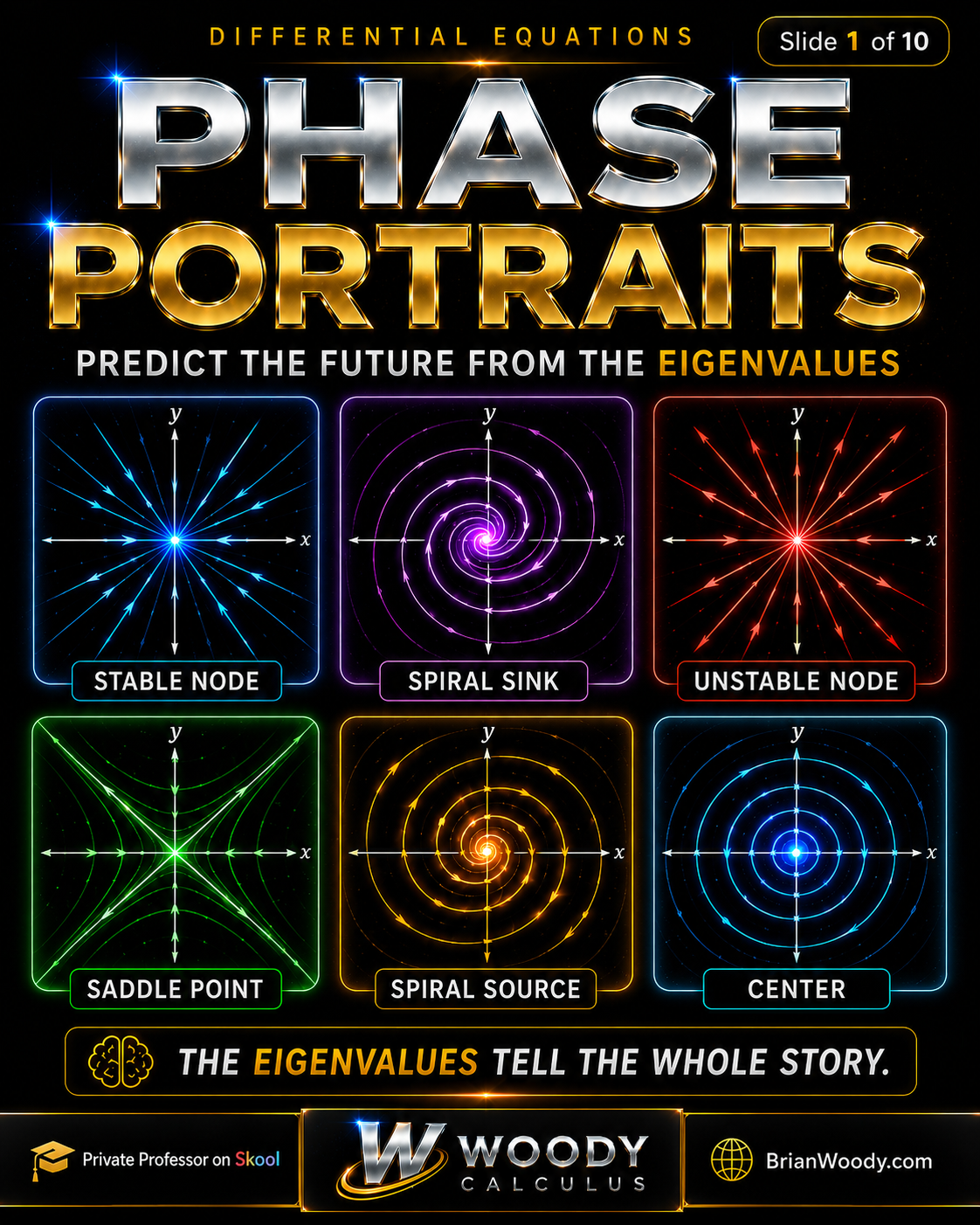
Phase Portraits Key Facts
- A phase portrait shows how solutions move through the phase plane.
- For \(\vec{x}^{\prime}=A\vec{x}\), eigenvalues determine growth, decay, and oscillation.
- Eigenvectors determine invariant straight-line directions.
- If both real eigenvalues are negative and distinct, the origin is a stable node.
- If both real eigenvalues are positive and distinct, the origin is an unstable node.
- If one real eigenvalue is positive and one is negative, the origin is a saddle point.
- If complex eigenvalues have negative real part, the phase portrait is a spiral sink.
- If complex eigenvalues have positive real part, the phase portrait is a spiral source.
- If eigenvalues are purely imaginary, the linear system has a center.
- If eigenvalues are repeated, you must check the number of independent eigenvectors.
This Woody Calculus lesson explains phase portraits in order: the system \(\vec{x}^{\prime}=A\vec{x}\), the eigenvalue workflow, stable nodes, unstable nodes, saddle points, spiral sinks, spiral sources, centers, repeated eigenvalues, worked examples, common mistakes, and exam-ready classification rules.
The Big Picture: From Matrix to Motion
A two-dimensional linear autonomous system has the form:
\vec{x}^{\prime}=A\vec{x}.
\]
Here, \(\vec{x}(t)\) is usually written as:
\vec{x}(t)=
\begin{bmatrix}
x(t)\\
y(t)
\end{bmatrix}.
\]
The matrix \(A\) controls the motion. The phase portrait is the picture of how solution curves move in the \(xy\)-plane.
The standard workflow is:
- Start with the system \(\vec{x}^{\prime}=A\vec{x}\).
- Find the eigenvalues from \(\det(A-\lambda I)=0\).
- Use the eigenvalues and eigenvectors to classify the equilibrium at the origin.
- Draw the phase portrait and predict stability.
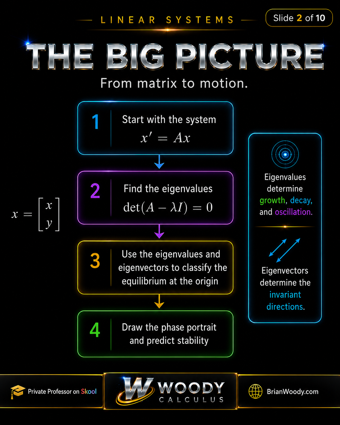
Why eigenvalues control the portrait
If \(A\vec{v}=\lambda\vec{v}\), then along the eigenvector direction \(\vec{v}\), solutions behave like:
\vec{x}(t)=c e^{\lambda t}\vec{v}.
\]
That formula explains the whole story:
- If \(\lambda<0\), then \(e^{\lambda t}\to 0\), so motion decays toward the origin.
- If \(\lambda>0\), then \(e^{\lambda t}\to \infty\), so motion grows away from the origin.
- If \(\lambda=a\pm bi\), the real part \(a\) controls growth or decay, while \(b\) creates rotation.
This is the same eigenvalue logic that appears in eigenvalues and eigenvectors in linear systems: the special directions reveal how the matrix moves the entire plane.
Phase Portrait Classification Cheat Sheet
For a two-dimensional linear system \(\vec{x}^{\prime}=A\vec{x}\), the eigenvalue pattern gives the classification:
| Eigenvalues | Phase Portrait | Stability | Main Idea |
|---|---|---|---|
| \(\lambda_1<0,\lambda_2<0\), real distinct | Stable node | Asymptotically stable | All nearby solutions approach the origin. |
| \(\lambda_1>0,\lambda_2>0\), real distinct | Unstable node | Unstable | Solutions move away from the origin. |
| \(\lambda_u>0,\lambda_s<0\) | Saddle point | Unstable | One eigendirection attracts; one repels. |
| \(\lambda=a\pm bi,\ a<0,\ b\ne 0\) | Spiral sink | Asymptotically stable | Solutions spiral into the origin. |
| \(\lambda=a\pm bi,\ a>0,\ b\ne 0\) | Spiral source | Unstable | Solutions spiral away from the origin. |
| \(\lambda=\pm bi,\ b\ne 0\) | Center | Neutrally stable in the linear system | Solutions form closed orbits. |
| \(\lambda_1=\lambda_2=\lambda\) | Repeated eigenvalue case | Depends on \(\lambda\) and eigenvectors | Check the number of independent eigenvectors. |
Trace and determinant shortcut
For a \(2\times 2\) matrix
A=
\begin{bmatrix}
a & b\\
c & d
\end{bmatrix},
\]
the characteristic polynomial can be written as:
\lambda^2-\operatorname{tr}(A)\lambda+\det(A)=0.
\]
Here,
\operatorname{tr}(A)=a+d,
\qquad
\det(A)=ad-bc.
\]
The determinant and trace help you quickly identify whether the eigenvalues are real, repeated, or complex. This is why many Differential Equations courses teach both the eigenvalue method and the trace-determinant plane.
Stable Node: Negative Real Eigenvalues
A stable node occurs when the system has two real, distinct, negative eigenvalues:
\lambda_1<0,\qquad \lambda_2<0. \]
Since both eigenvalues are negative, both exponential factors decay:
e^{\lambda_1 t}\to 0,
\qquad
e^{\lambda_2 t}\to 0
\qquad
\text{as }t\to\infty.
\]
Therefore, nearby solutions approach the equilibrium at the origin. The origin is locally asymptotically stable.
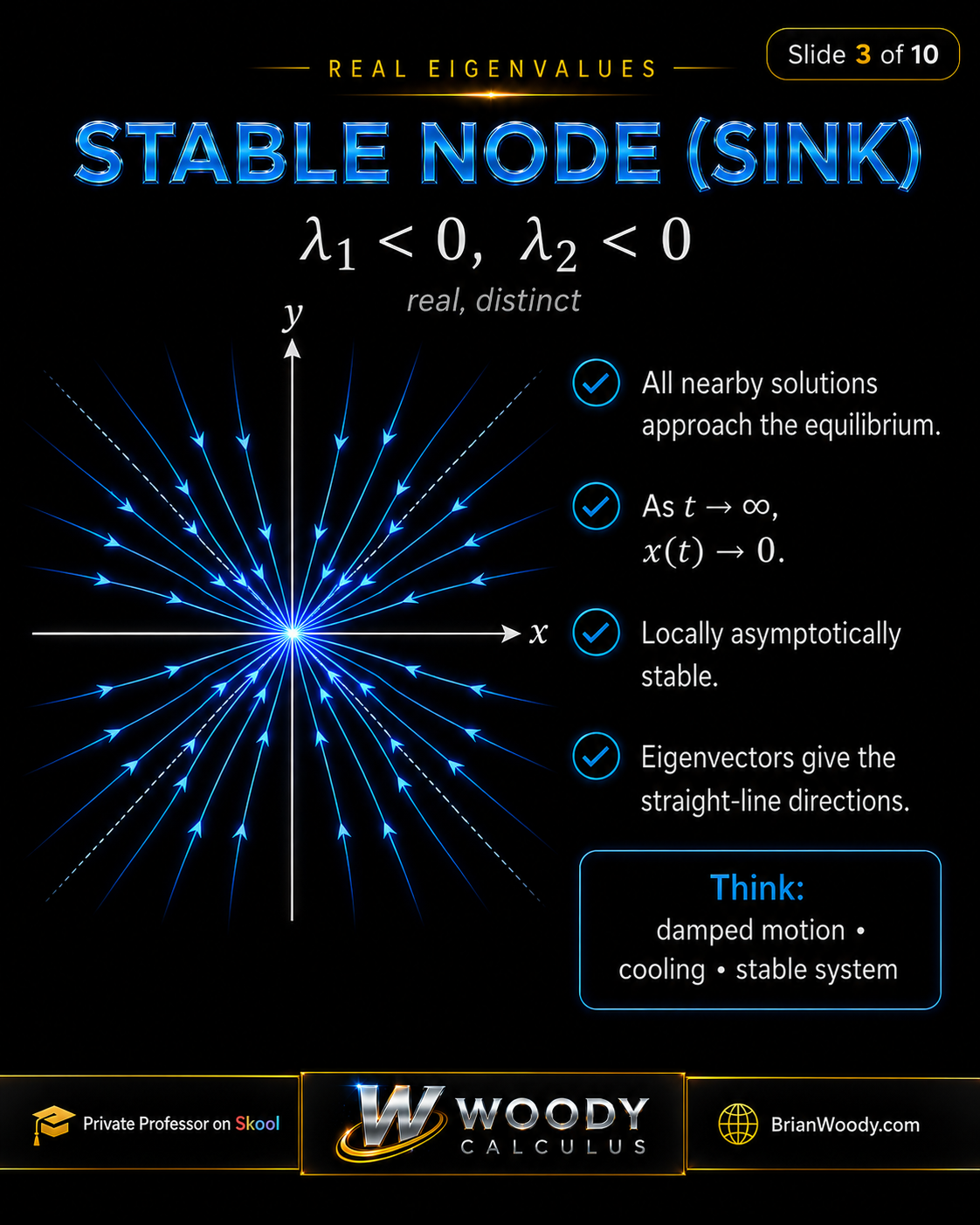
How to think about a stable node
A stable node represents damping, cooling, decay, or a stable system. The eigenvectors give the straight-line directions. Other nearby trajectories curve toward the origin while becoming tangent to the slowest-decaying eigendirection.
This is a major exam topic in Differential Equations because it connects algebra, geometry, and stability in one picture.
Unstable Node: Positive Real Eigenvalues
An unstable node, also called a source, occurs when both real, distinct eigenvalues are positive:
\lambda_1>0,\qquad \lambda_2>0.
\]
Since both eigenvalues are positive, both exponential factors grow:
e^{\lambda_1 t}\to \infty,
\qquad
e^{\lambda_2 t}\to \infty
\qquad
\text{as }t\to\infty.
\]
So nonzero nearby solutions move away from the origin. The equilibrium is unstable.
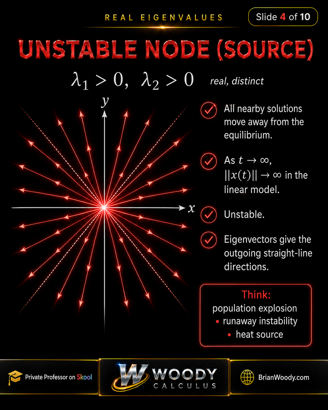
How to think about an unstable node
An unstable node represents runaway growth, population explosion, heat sources, or instability. The eigenvectors give the outgoing straight-line directions.
The classification is the exact opposite of the stable node: the signs of the eigenvalues reverse the direction of time behavior.
Saddle Point: One Positive and One Negative Eigenvalue
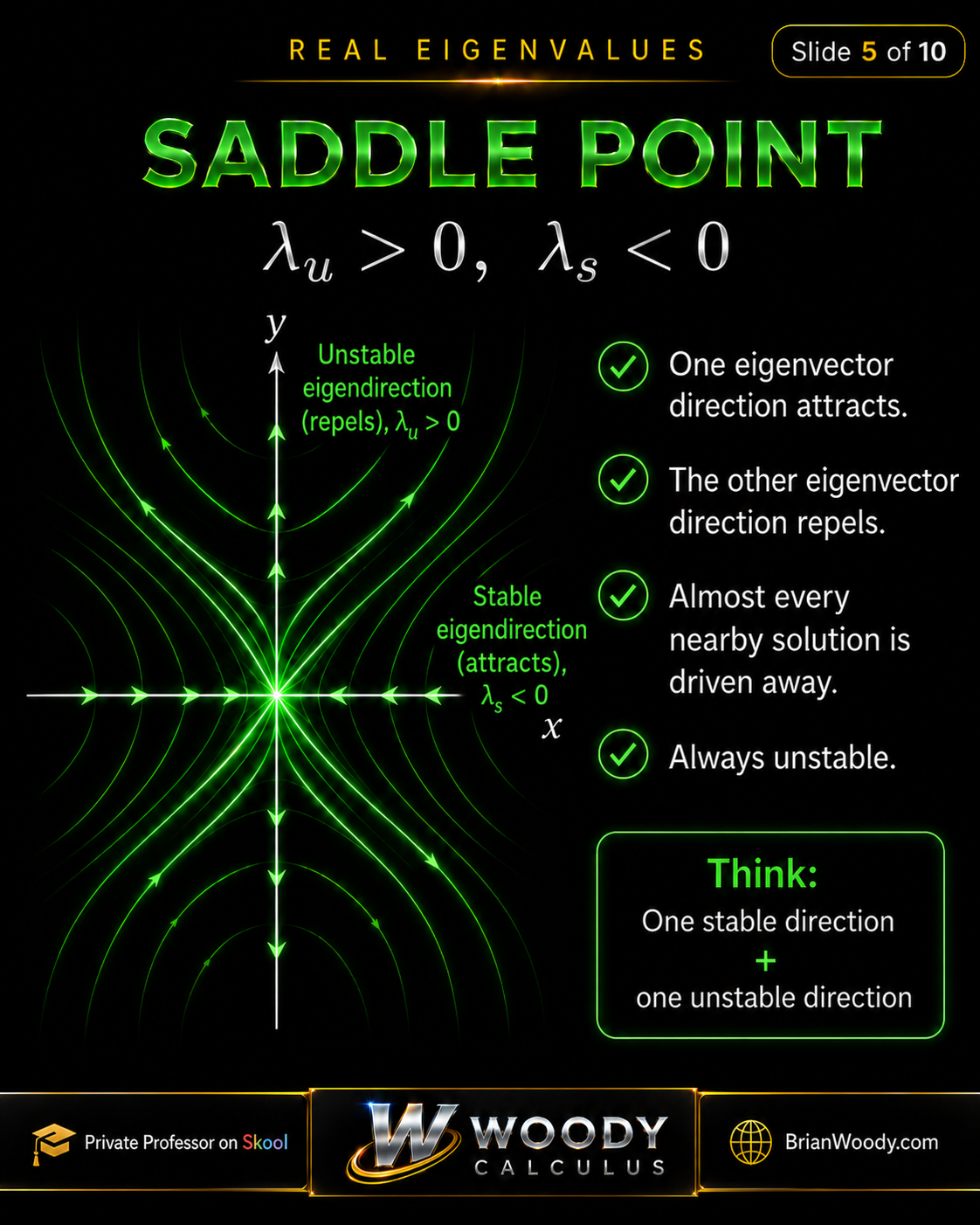
A saddle point occurs when the real eigenvalues have opposite signs:
\lambda_u>0,\qquad \lambda_s<0. \]
The positive eigenvalue creates an unstable eigendirection, while the negative eigenvalue creates a stable eigendirection.
Along the stable eigendirection, solutions approach the origin. Along the unstable eigendirection, solutions move away from the origin. Almost every nearby solution is eventually driven away.
Why saddle points are always unstable
A saddle point is always unstable because there is at least one direction in which solutions move away from equilibrium. Even though one eigendirection attracts, the repelling direction makes the equilibrium unstable.
This same idea appears in chaos theory and the Lorenz system, where stable and unstable directions help create complicated long-term behavior.
Spiral Sink: Complex Eigenvalues with Negative Real Part
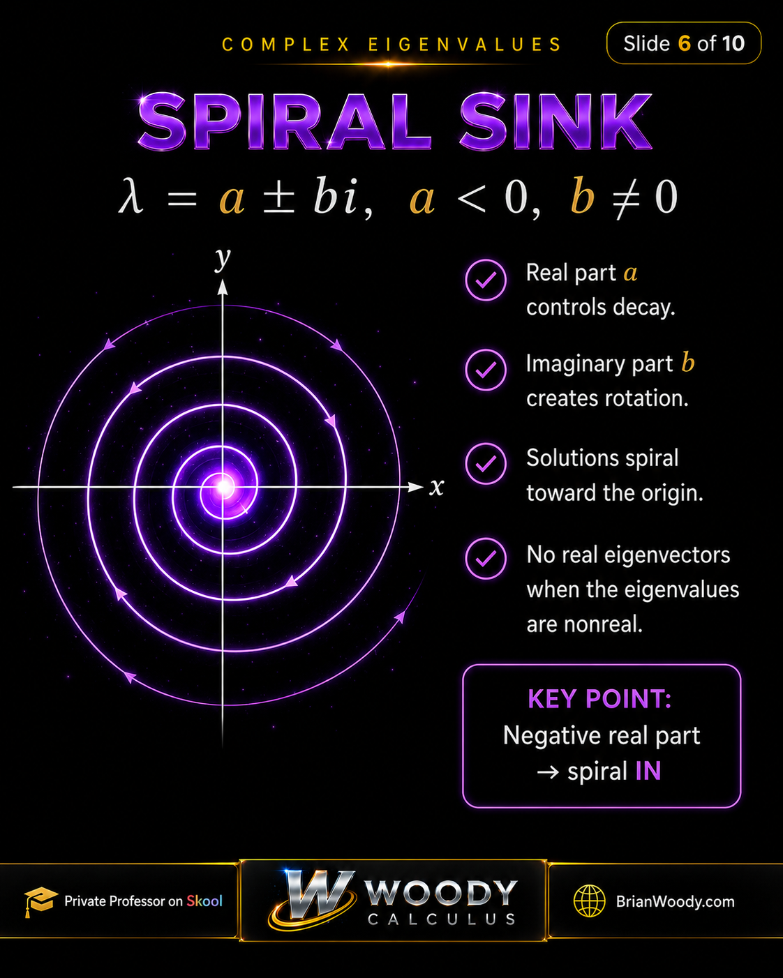
A spiral sink occurs when the eigenvalues are complex conjugates:
\lambda=a\pm bi,
\qquad
a<0, \qquad b\ne 0. \]
The real part \(a\) controls decay. Since \(a<0\), the solutions decay toward the origin. The imaginary part \(b\) creates rotation.
So the solutions spiral inward.
No real eigenvectors in the spiral case
When the eigenvalues are nonreal complex numbers, the real matrix \(A\) has no real eigenvectors. That is why the portrait does not have straight-line eigendirections in the phase plane.
The real part controls whether the spiral moves inward or outward. The imaginary part controls the rotation.
Spiral Source: Complex Eigenvalues with Positive Real Part
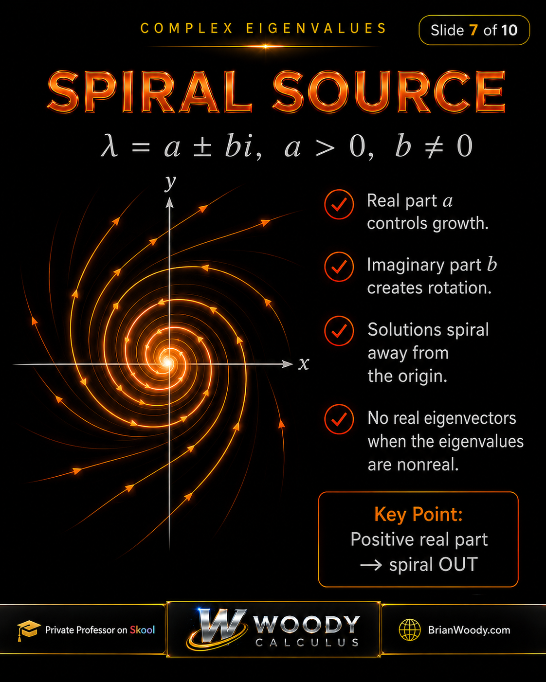
A spiral source occurs when the eigenvalues are:
\lambda=a\pm bi,
\qquad
a>0,
\qquad
b\ne 0.
\]
The real part \(a\) controls growth. Since \(a>0\), the exponential factor grows, and solutions spiral away from the origin.
Spiral sink versus spiral source
The difference between a spiral sink and a spiral source is the sign of the real part:
- If \(a<0\), solutions spiral inward.
- If \(a>0\), solutions spiral outward.
This is why students should say the rule out loud: real part controls growth or decay; imaginary part creates rotation.
Center: Purely Imaginary Eigenvalues
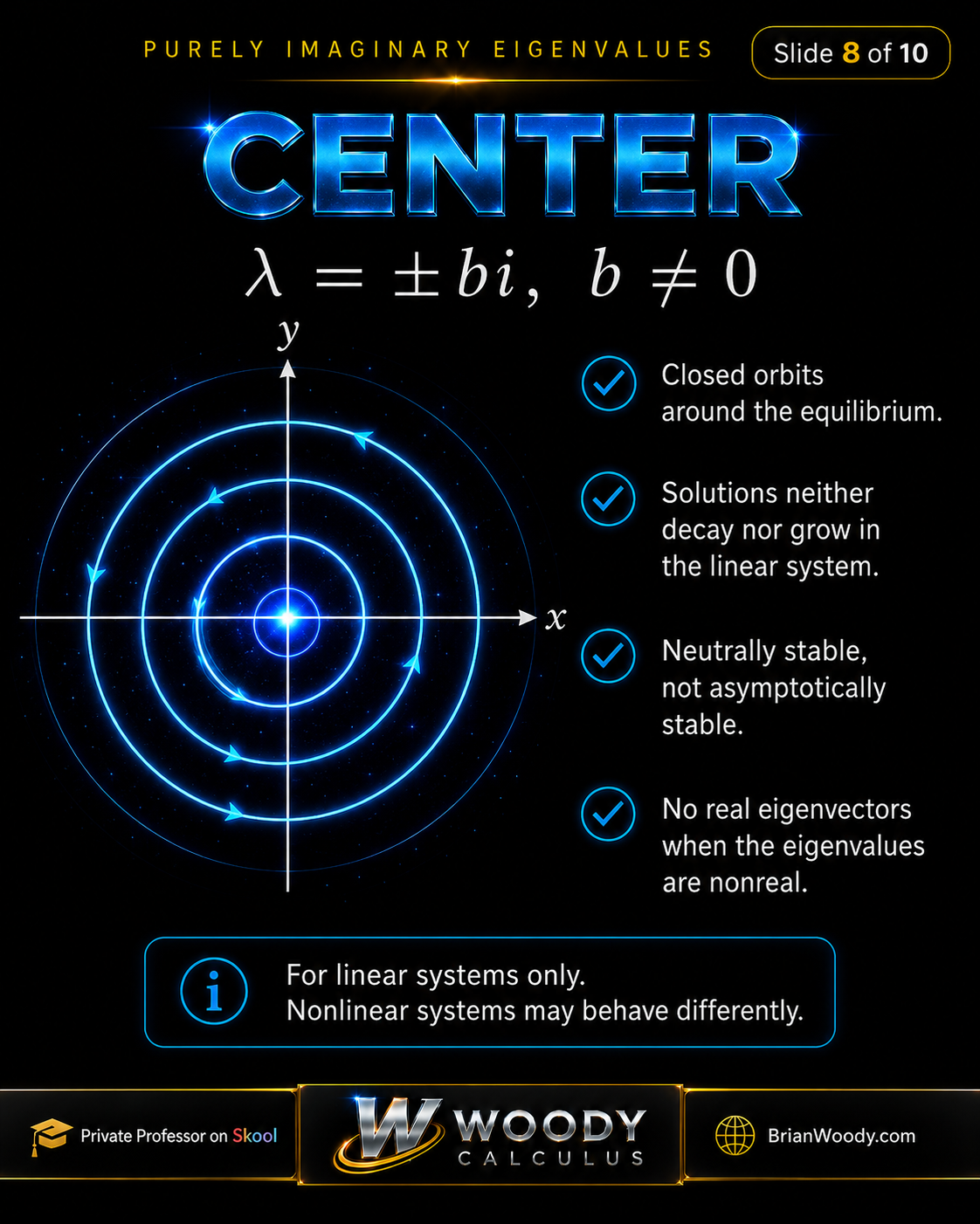
A center occurs in the linear system when the eigenvalues are purely imaginary:
\lambda=\pm bi,
\qquad
b\ne 0.
\]
There is no real part. That means solutions neither decay nor grow in the linear system. Instead, the trajectories form closed orbits around the equilibrium.
Important warning for nonlinear systems
For linear systems, purely imaginary eigenvalues produce a center. But nonlinear systems may behave differently. A nonlinear system with purely imaginary eigenvalues at the linearized level may become a spiral sink, spiral source, center, or something more subtle depending on the nonlinear terms.
This is why hypotheses matter. In advanced courses such as Real Analysis and nonlinear Differential Equations, similar-looking conditions can lead to different conclusions.
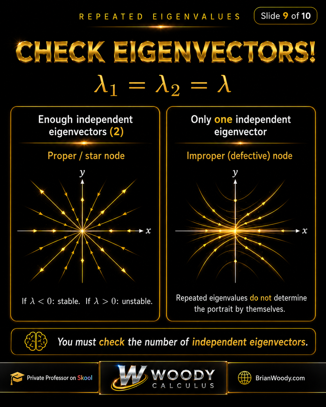
Repeated Eigenvalues: Check Eigenvectors
Repeated eigenvalues require extra care. If:
\lambda_1=\lambda_2=\lambda,
\]
then the eigenvalue alone does not always determine the phase portrait. You must check the number of independent eigenvectors.
If there are enough independent eigenvectors, the system has a proper node or star node. If there is only one independent eigenvector, the system has an improper or defective node.
Stable or unstable repeated eigenvalue cases
The sign of the repeated eigenvalue still matters:
- If \(\lambda<0\), the repeated-eigenvalue node is stable.
- If \(\lambda>0\), the repeated-eigenvalue node is unstable.
But the shape of the portrait depends on whether you have enough independent eigenvectors.
Worked Examples
Worked Example 1: Stable node
Classify the system:
\vec{x}^{\prime}=
\begin{bmatrix}
-2 & 0\\
0 & -3
\end{bmatrix}
\vec{x}.
\]
The matrix is diagonal, so the eigenvalues are:
\lambda_1=-2,\qquad \lambda_2=-3.
\]
Both eigenvalues are real, distinct, and negative. Therefore, the origin is a stable node.
As \(t\to\infty\), both components decay to \(0\), so \(\vec{x}(t)\to \vec{0}\).
Worked Example 2: Saddle point
Classify the system:
\vec{x}^{\prime}=
\begin{bmatrix}
1 & 0\\
0 & -2
\end{bmatrix}
\vec{x}.
\]
The eigenvalues are:
\lambda_1=1,\qquad \lambda_2=-2.
\]
One eigenvalue is positive and one is negative. Therefore, the origin is a saddle point.
The \(y\)-direction decays because \(-2<0\), while the \(x\)-direction grows because \(1>0\). The equilibrium is unstable.
Worked Example 3: Spiral sink
Classify the system:
\vec{x}^{\prime}=
\begin{bmatrix}
-1 & -4\\
4 & -1
\end{bmatrix}
\vec{x}.
\]
The trace and determinant are:
\operatorname{tr}(A)=-2,
\qquad
\det(A)=17.
\]
The characteristic polynomial is:
\lambda^2+2\lambda+17=0.
\]
Using the quadratic formula:
\lambda=\frac{-2\pm\sqrt{4-68}}{2}
=
\frac{-2\pm 8i}{2}
=
-1\pm 4i.
\]
The eigenvalues are complex with negative real part. Therefore, the origin is a spiral sink.
Worked Example 4: Center
Classify the system:
\vec{x}^{\prime}=
\begin{bmatrix}
0 & -2\\
2 & 0
\end{bmatrix}
\vec{x}.
\]
The characteristic polynomial is:
\lambda^2+4=0.
\]
So:
\lambda=\pm 2i.
\]
The eigenvalues are purely imaginary. Therefore, the linear system has a center. The solutions form closed orbits around the origin.
Worked Example 5: Repeated eigenvalue with one eigenvector
Classify:
A=
\begin{bmatrix}
-1 & 1\\
0 & -1
\end{bmatrix}.
\]
The only eigenvalue is:
\lambda=-1.
\]
Because \(A\) is not diagonal and has only one independent eigenvector, this is a defective repeated-eigenvalue case. Since \(\lambda<0\), the origin is a stable improper node.
Common Mistakes with Phase Portraits
Mistake 1: Forgetting that eigenvectors give directions
Eigenvalues classify growth, decay, and oscillation. Eigenvectors give the invariant directions. For real eigenvalues, the eigenvectors are the straight-line solution directions in the phase plane.
Mistake 2: Calling every complex case a center
Complex eigenvalues only give a center when the real part is zero. If \(\lambda=a\pm bi\) with \(a<0\), the portrait is a spiral sink. If \(a>0\), the portrait is a spiral source.
Mistake 3: Thinking a saddle point is partly stable
A saddle has one stable direction, but the equilibrium itself is unstable because nearby points not exactly on the stable eigendirection move away.
Mistake 4: Ignoring repeated eigenvalues
When eigenvalues repeat, you must check the number of independent eigenvectors. Repeated eigenvalues alone do not determine the phase portrait.
Mistake 5: Applying the linear center rule to every nonlinear system
Purely imaginary eigenvalues give a center for linear systems. Nonlinear systems may behave differently, so the nonlinear terms matter.
Key Takeaways
- To classify a phase portrait, start by finding the eigenvalues of \(A\).
- If both eigenvalues are real and negative, you have a stable node.
- If both eigenvalues are real and positive, you have an unstable node.
- If eigenvalues have opposite signs, you have a saddle point.
- If eigenvalues are complex with negative real part, you have a spiral sink.
- If eigenvalues are complex with positive real part, you have a spiral source.
- If eigenvalues are purely imaginary, you have a center for the linear system.
- For repeated eigenvalues, always check the number of independent eigenvectors.
Phase Portraits FAQ
What is a phase portrait in Differential Equations?
A phase portrait is a geometric picture showing how solutions of a differential equation system move through the phase plane.
How do eigenvalues determine a phase portrait?
Eigenvalues determine whether solutions grow, decay, rotate, or combine these behaviors. Real eigenvalues create node or saddle behavior, while complex eigenvalues create spirals or centers.
What is a stable node?
A stable node occurs when both real eigenvalues are negative. Nearby solutions approach the equilibrium as time increases.
What is an unstable node?
An unstable node occurs when both real eigenvalues are positive. Nearby nonzero solutions move away from the equilibrium as time increases.
Why is a saddle point unstable?
A saddle point is unstable because one eigendirection repels solutions away from the equilibrium, even though another eigendirection attracts.
What causes a spiral sink?
A spiral sink occurs when the eigenvalues are complex with negative real part. The negative real part creates decay, and the imaginary part creates rotation.
What causes a spiral source?
A spiral source occurs when the eigenvalues are complex with positive real part. The positive real part creates growth, and the imaginary part creates rotation.
What is a center in a linear system?
A center occurs when the eigenvalues are purely imaginary. Solutions form closed orbits around the equilibrium and are neutrally stable in the linear model.
What should I do with repeated eigenvalues?
When eigenvalues are repeated, check the number of independent eigenvectors. Enough independent eigenvectors give a proper or star node, while one independent eigenvector gives an improper or defective node.
Master Phase Portraits with Woody Calculus
Understanding phase portraits begins with mastering the mathematics behind them: Differential Equations, eigenvalues, eigenvectors, matrix systems, phase planes, stability, and linearization.
Woody Calculus provides structured, university-level instruction designed to build formula fluency, genuine mathematical understanding, and exam-ready execution. The goal is not just to recognize formulas. The goal is to know when to use them, how to set them up cleanly, how to interpret the answer, and how to write complete solutions under pressure.
A phase portrait turns eigenvalues into motion. Once you can read the eigenvalues, you can predict the future of the system.
— Brian M. Woody
Woody Calculus CTA
If you are studying Differential Equations, Calculus 2, Calculus 3, Linear Algebra, Abstract Algebra, Real Analysis, Number Theory, Topology, or advanced mathematics, Woody Calculus can help you build a serious system for learning.
Visit BrianWoody.com for Woody Calculus visual mathematics lessons covering free mathematical essays, visual lessons, exam-focused resources, and advanced university math support.
For structured training, join the Woody Calculus Mastery Lab for university mathematics, where students learn through clean definitions, clean setup, formula fluency, pattern recognition, rewriting perfect solutions, and saying each step out loud until the method becomes automatic.
Join Woody Calculus Mastery Lab on Skool
Related Woody Calculus Mathematical Essays
Explore more Woody Calculus visual lessons and deep-dive mathematical essays connecting Differential Equations, Calculus 2, Calculus 3, Linear Algebra, Real Analysis, Abstract Algebra, Number Theory, Topology, phase portraits, eigenvalues, and peak performance study methods.
- How to Learn Calculus and Advanced Mathematics: A Peak Performance Study Guide
- Resonance Explained for Differential Equations: Forced Oscillations and Natural Frequency
- How Differential Equations Give Rise to Chaos Theory
- Chaos Theory Explained: Butterfly Effect, Lorenz System, and Lyapunov Exponents
- Eigenvalues and Eigenvectors Explained: The Special Directions That Unlock Linear Algebra
- The Determinant Explained: The Number That Measures How a Matrix Changes Space
- Laplace Transforms Explained: Turning Differential Equations Into Algebra
- The Jacobian Explained: The Hidden Scale Factor in Calculus III
- Line Integrals and Vector Fields: What They Measure in Calculus 3
- Green’s Theorem Explained: Why a Boundary Knows Everything Inside
- Stokes’ Theorem Explained: Why the Edge Knows the Surface
- Fourier Series Explained: Harmonics, Sound, Heat, and Quantum Mechanics
- View All Woody Calculus Blog Posts
Related University Math Help Pages
Woody Calculus supports students at major universities with structured help in Differential Equations, Calculus II, Calculus III, Linear Algebra, Real Analysis, Abstract Algebra, Number Theory, Topology, and advanced mathematics. For the full list of supported schools, visit the University Calculus Tutor Hub.
- University Calculus Tutor Hub
- MIT Calculus Tutor
- Purdue University Calculus Tutor
- University of Florida Calculus Tutor
- Colorado State University Calculus Help
- UCF Calculus Tutor
- Georgia Tech Calculus Tutor
- University of Michigan Calculus Tutor
- University of Nevada, Reno Calculus Tutor
- University of Wisconsin Calculus Tutor
Trusted by Students Nationwide
The Woody Calculus Mastery Lab gives university students access to structured mathematics support, written solutions, video lessons, exam-focused training, proof-based lessons, and expert guidance from Brian M. Woody.
Students use Woody Calculus for Differential Equations, Calculus II, Calculus III, Linear Algebra, Abstract Algebra, Real Analysis, Number Theory, Topology, and other advanced mathematics courses.