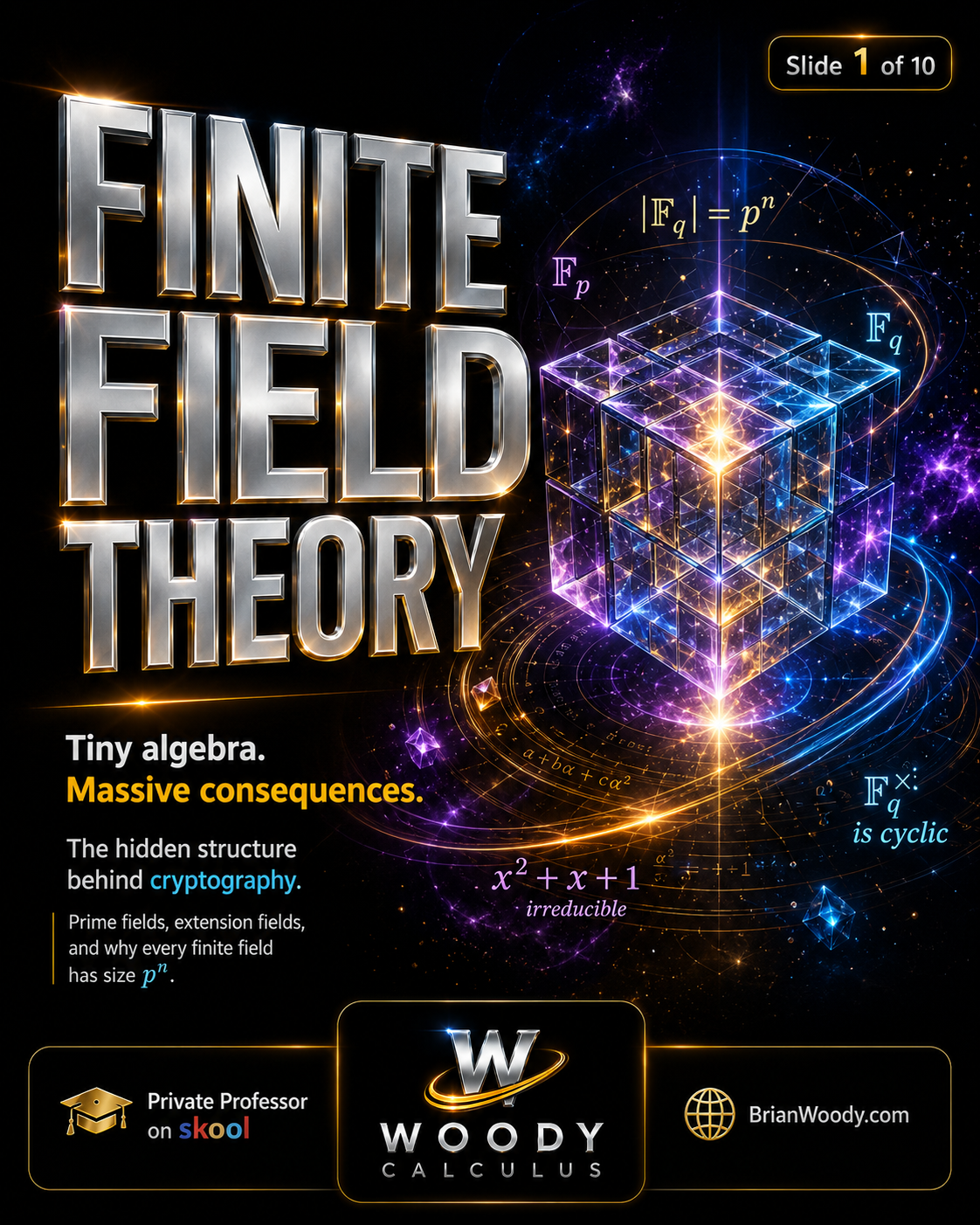
Finite field theory looks abstract until you realize it is part of the mathematics holding modern technology together. Finite fields appear in cryptography, AES encryption, elliptic curve cryptography, Reed–Solomon error correction, QR codes, secure communication, and modern coding theory.
A finite field is a tiny number system where addition, subtraction, multiplication, and division still work, but everything lives inside a finite universe.
The central theorem is one of the most important facts in Abstract Algebra:
|\mathbb{F}_q|=q=p^n.
\]
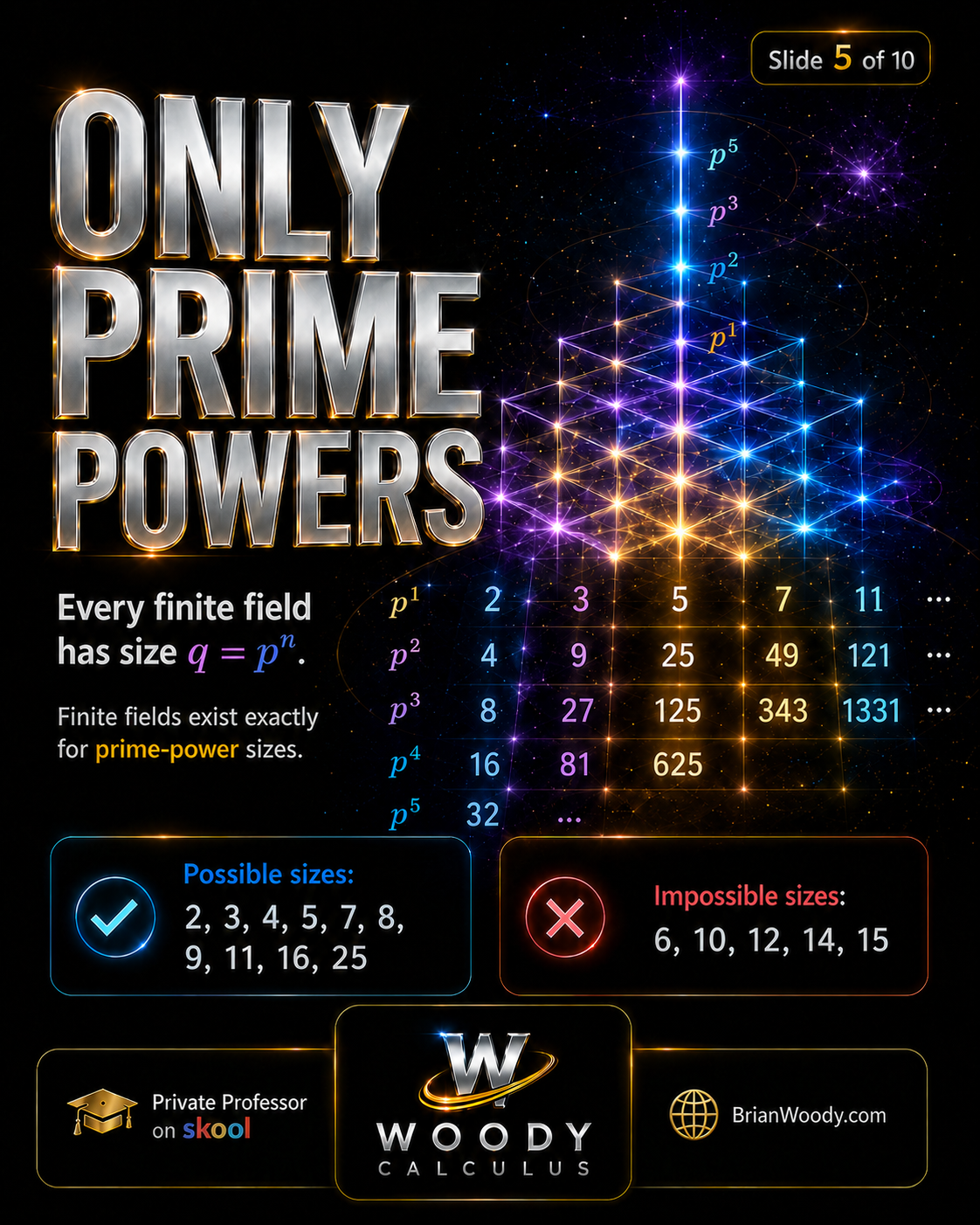
That means every finite field has prime-power size. Finite fields can have \(2,3,4,5,7,8,9,11,16,25,\ldots\) elements, but not \(6,10,12,14,15,\ldots\) elements.
Prime powers only.
Finite Field Theory Key Facts
- A finite field is a field with finitely many elements.
- Every finite field has size \(q=p^n\), where \(p\) is prime and \(n\) is a positive integer.
- Prime fields have the form \(\mathbb{F}_p=\{0,1,2,\ldots,p-1\}\).
- Extension fields are built using irreducible polynomials over prime fields.
- The nonzero elements of a finite field form a cyclic multiplicative group.
- Finite fields power AES encryption, elliptic curve cryptography, Reed–Solomon codes, QR codes, and data recovery.
- Finite field theory connects directly to field extensions, Galois Theory, Galois groups, and modern finite-field research.
Quick Summary
Finite field theory studies fields with finitely many elements. Every finite field has size \(p^n\), where \(p\) is prime. Prime fields use arithmetic modulo \(p\), while extension fields are built from irreducible polynomials. These structures are essential in cryptography, error correction, coding theory, and Brian M. Woody’s finite-field research on permutation polynomials over \(\mathbb{F}_{q^2}\).
This Woody Calculus visual lesson explains finite field theory in order: what a field is, why prime fields matter, why composite moduli fail, why every finite field has size \(p^n\), how extension fields are built from irreducible polynomials, why finite field multiplication is cyclic, and why finite fields power cryptography and communication.
What Is Finite Field Theory?
Finite field theory studies fields with finitely many elements. These fields are also called Galois fields, and they are usually written as \(\mathbb{F}_q\) or \(GF(q)\), where \(q\) is the number of elements in the field.
The surprising part is that not every finite size is possible. A finite field must have size
q=p^n,
\]
where \(p\) is prime and \(n\) is a positive integer.
This theorem is the reason finite fields can have \(4=2^2\), \(8=2^3\), \(9=3^2\), and \(25=5^2\) elements, but cannot have \(6\), \(10\), \(12\), \(14\), or \(15\) elements.
Finite field theory is small algebra with massive consequences. It connects modular arithmetic, polynomial algebra, group theory, field extensions, Galois Theory, cryptography, coding theory, and digital communication.
What Is a Field?
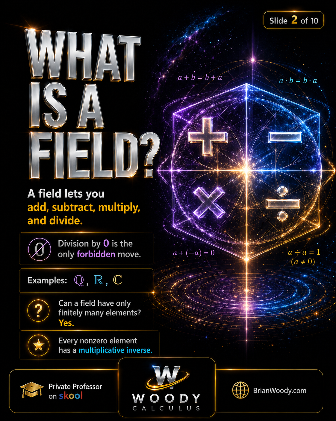
A field is a number system where you can add, subtract, multiply, and divide, except that division by zero is forbidden.
Examples of familiar fields include:
- \(\mathbb{Q}\), the rational numbers
- \(\mathbb{R}\), the real numbers
- \(\mathbb{C}\), the complex numbers
The key rule is that every nonzero element must have a multiplicative inverse. In other words, if \(a\ne 0\), then there must be some element \(a^{-1}\) such that
a\cdot a^{-1}=1.
\]
This inverse rule is what makes division possible. If an algebraic system has addition and multiplication but nonzero elements do not always have inverses, then it is not a field.
A finite field is simply a field with finitely many elements.
Prime Fields
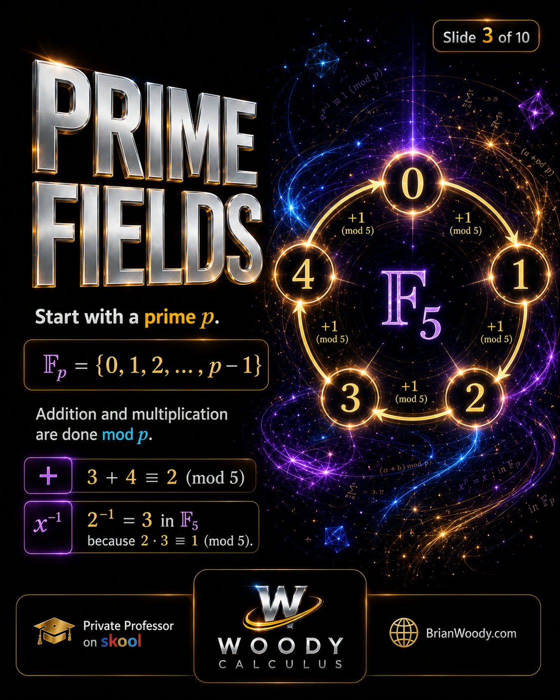
The simplest finite fields are prime fields. Start with a prime number \(p\). The prime field \(\mathbb{F}_p\) has elements
\mathbb{F}_p=\{0,1,2,\ldots,p-1\}.
\]
Addition and multiplication are done modulo \(p\).
For example, in \(\mathbb{F}_5\),
3+4=7\equiv 2 \pmod 5.
\]
Also, \(2^{-1}=3\) in \(\mathbb{F}_5\), because
2\cdot 3=6\equiv 1 \pmod 5.
\]
So \(3\) is the multiplicative inverse of \(2\) modulo \(5\).
Prime fields are the starting point for finite field theory. They are built from modular arithmetic, but the prime condition is essential.
Why Prime Matters
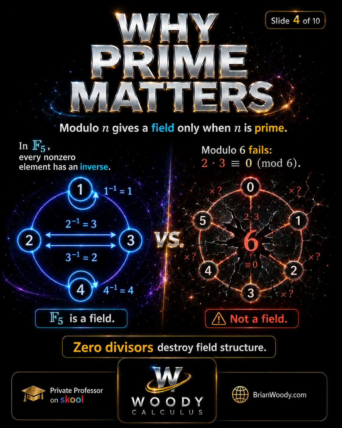
Modulo \(n\) arithmetic gives a field only when \(n\) is prime.
For example, modulo \(5\) works because \(5\) is prime. Every nonzero element in \(\mathbb{F}_5\) has a multiplicative inverse:
- \(1^{-1}=1\)
- \(2^{-1}=3\)
- \(3^{-1}=2\)
- \(4^{-1}=4\)
But modulo \(6\) fails.
In modulo \(6\),
2\cdot 3=6\equiv 0 \pmod 6.
\]
Here \(2\) and \(3\) are both nonzero, but their product is zero. These are called zero divisors.
Zero divisors destroy field structure because nonzero elements with zero products cannot have multiplicative inverses.
That is why \(\mathbb{F}_5\) is a field, but arithmetic modulo \(6\) is not.
Only Prime Powers
The fundamental finite field theorem says:
|\mathbb{F}_q|=q=p^n.
\]
Every finite field has prime-power size. Conversely, for every prime power \(p^n\), there exists a finite field with \(p^n\) elements, unique up to isomorphism.
This means finite fields exist exactly for prime-power sizes.
Possible finite field sizes include:
2,3,4,5,7,8,9,11,16,25,\ldots
\]
because these are prime powers:
- \(2=2^1\)
- \(3=3^1\)
- \(4=2^2\)
- \(8=2^3\)
- \(9=3^2\)
- \(16=2^4\)
- \(25=5^2\)
Impossible finite field sizes include:
6,10,12,14,15,\ldots
\]
because these are not prime powers.
This is one of the big turning points in abstract algebra: finite fields are not arbitrary. Their sizes are rigidly controlled by prime powers.
Extension Fields
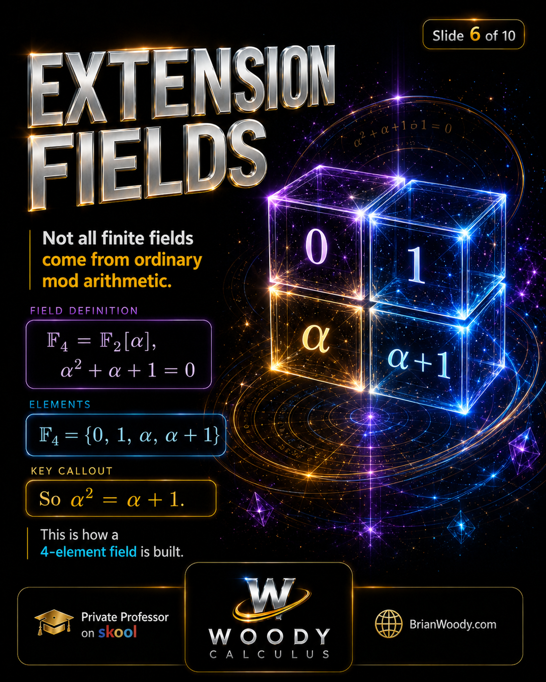
Not all finite fields come from ordinary modular arithmetic.
For example, there is a field with \(4\) elements, but it is not simply arithmetic modulo \(4\). Modulo \(4\) is not a field because \(2\cdot 2=0 \pmod 4\), so \(2\) is a zero divisor.
Instead, the field with \(4\) elements is built as an extension field of \(\mathbb{F}_2\).
One way to build it is:
\mathbb{F}_4=\mathbb{F}_2[\alpha],
\qquad
\alpha^2+\alpha+1=0.
\]
The elements are
\mathbb{F}_4=\{0,1,\alpha,\alpha+1\}.
\]
Because \(\alpha^2+\alpha+1=0\), and arithmetic is happening in characteristic \(2\), we get
\alpha^2=\alpha+1.
\]
This relation lets us reduce higher powers of \(\alpha\) back into the four-element set.
This is how a \(4\)-element field is built. To see the broader theory of building larger fields by adjoining roots, read Field Extensions Explained: When Numbers Need a Bigger Universe.
Irreducible Polynomials
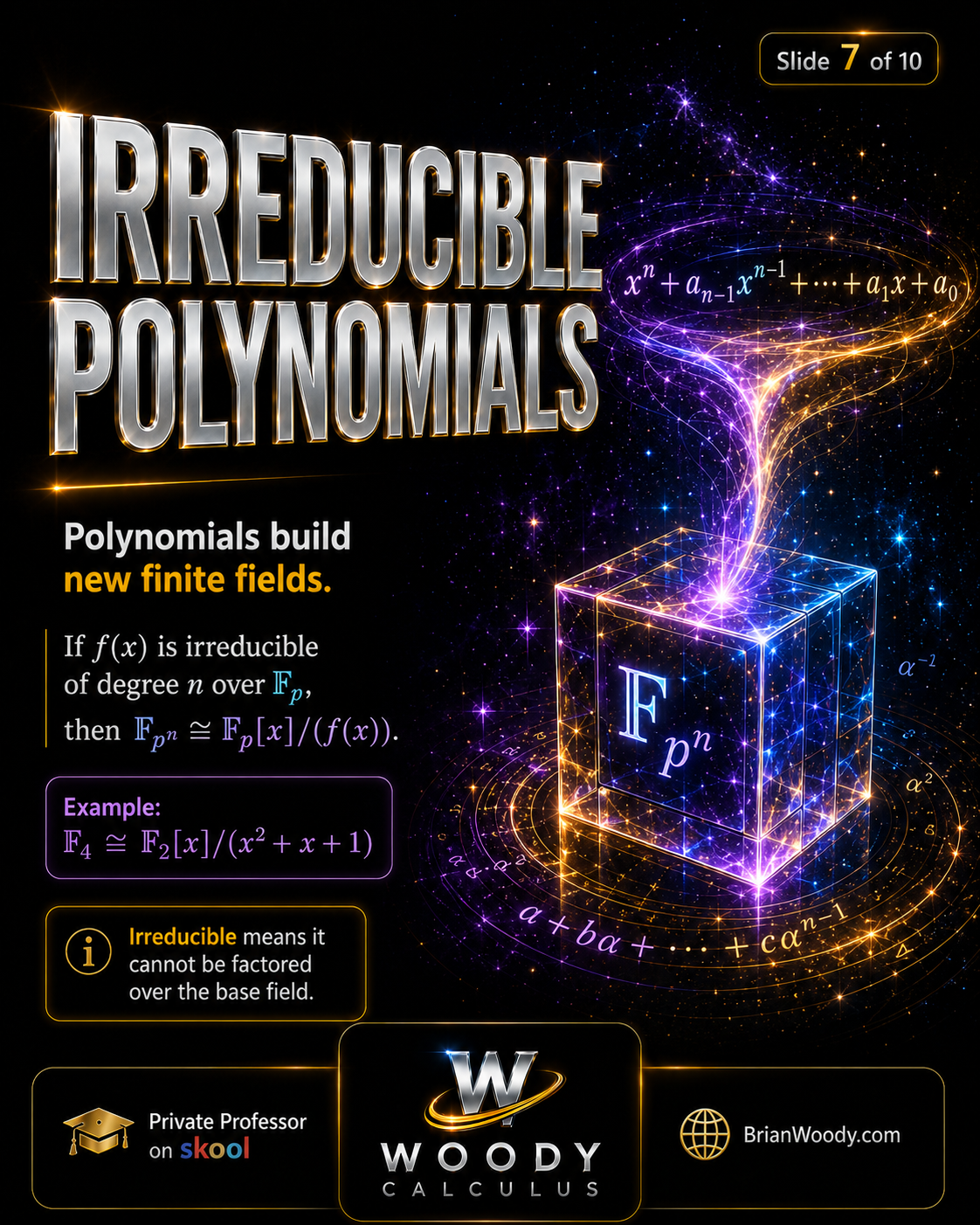
Irreducible polynomials are the engines that build extension fields.
A polynomial is irreducible over a field if it cannot be factored into lower-degree polynomials over that field.
If \(f(x)\) is irreducible of degree \(n\) over \(\mathbb{F}_p\), then
\mathbb{F}_{p^n}\cong \mathbb{F}_p[x]/(f(x)).
\]
This means we build a new field by taking polynomials over \(\mathbb{F}_p\) and reducing them modulo the irreducible polynomial \(f(x)\).
For example,
\mathbb{F}_4\cong \mathbb{F}_2[x]/(x^2+x+1).
\]
The polynomial \(x^2+x+1\) is irreducible over \(\mathbb{F}_2\), so quotienting by it creates a field with \(2^2=4\) elements.
This is the general construction behind finite fields of size \(p^n\). The quotient notation here is an early glimpse of quotient structures in algebra; for the group-theory version, read Quotient Groups Explained: Cosets, Normal Subgroups, and the First Isomorphism Theorem.
Cyclic Multiplication
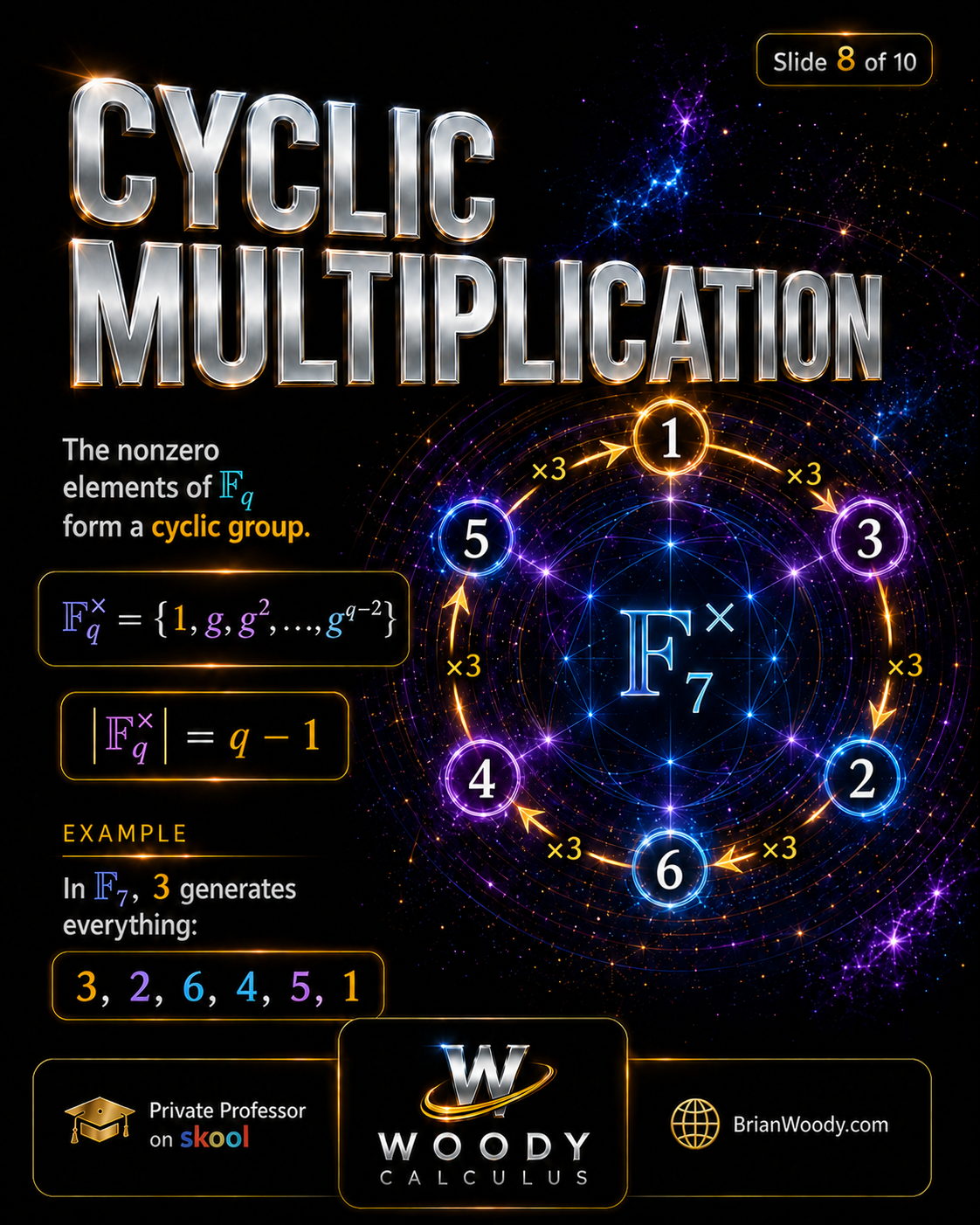
The nonzero elements of a finite field form a multiplicative group.
Even more beautifully, that group is always cyclic:
\mathbb{F}_q^\times=\{1,g,g^2,\ldots,g^{q-2}\},
\]
and
|\mathbb{F}_q^\times|=q-1.
\]
The element \(g\) is called a generator or primitive element. Repeated multiplication by \(g\) cycles through every nonzero element of the field.
For example, in \(\mathbb{F}_7\), the number \(3\) generates every nonzero element:
3,2,6,4,5,1.
\]
Here is the cycle:
- \(3^1\equiv 3 \pmod 7\)
- \(3^2\equiv 2 \pmod 7\)
- \(3^3\equiv 6 \pmod 7\)
- \(3^4\equiv 4 \pmod 7\)
- \(3^5\equiv 5 \pmod 7\)
- \(3^6\equiv 1 \pmod 7\)
So \(3\) generates \(\mathbb{F}_7^\times\).
This cyclic structure is one of the reasons finite fields are so powerful in cryptography, coding theory, and finite-field polynomial research.
Why Finite Fields Matter
Finite fields matter because they are the algebra behind modern security, communication, and error correction.
Here are three major examples.
AES Encryption
The Advanced Encryption Standard uses arithmetic in
GF(2^8).
\]
This is a finite field with \(256\) elements. The field structure makes it possible to perform algebraic operations that are reversible, structured, and secure.
Elliptic Curve Cryptography
Elliptic curve cryptography often works over finite fields. Points on elliptic curves are combined using algebraic rules, and the finite field structure controls the arithmetic.
This is one of the reasons finite fields are central in modern public-key cryptography.
Reed–Solomon Codes and QR Codes
Reed–Solomon codes use finite fields to detect and correct errors. These codes appear in QR codes, CDs, DVDs, satellite communication, and data recovery.
Finite fields make it possible to recover data even when part of the message has been damaged.
This is where abstract algebra stops feeling abstract and starts looking like the hidden operating system behind technology. For another application-facing lesson, see Blockchain Mathematics Explained: Hash Functions, Cryptography, AI, and Consensus.

Connection to Brian Woody’s Finite Field Research
Finite field theory is also the foundation for Brian M. Woody’s current research on permutation polynomials, reciprocal quadrinomials, Dickson trace curves, roots of unity, unit-circle reductions, and polynomial classification over \(\mathbb{F}_{q^2}\).
- Brian M. Woody Research Hub
- Finite Field Permutation Polynomial Research
- Dickson Trace Curves and Reciprocal Quadrinomials over Finite Fields
- Official arXiv Record: arXiv:2607.01267
Students who want to understand this research should build a foundation in finite fields, field extensions, Galois Theory, the Galois group of \(x^3-2\), and quotient groups.
Key Takeaways
- A field allows addition, subtraction, multiplication, and division by nonzero elements.
- A finite field is a field with finitely many elements.
- The prime field \(\mathbb{F}_p\) uses arithmetic modulo a prime \(p\).
- Modulo \(n\) gives a field only when \(n\) is prime.
- Every finite field has size \(q=p^n\).
- Finite fields exist exactly for prime-power sizes.
- Extension fields are built using irreducible polynomials.
- The nonzero elements of a finite field form a cyclic multiplicative group.
- Finite fields power AES encryption, elliptic curve cryptography, Reed–Solomon codes, QR codes, and data recovery.
- Finite fields also support modern research on permutation polynomials and reciprocal quadrinomials over \(\mathbb{F}_{q^2}\).
Finite Field Theory FAQ
What is a finite field?
A finite field is a field with finitely many elements. It supports addition, subtraction, multiplication, and division by nonzero elements, all inside a finite set.
Why must a finite field have size \(p^n\)?
Every finite field has prime characteristic \(p\), which means it contains a copy of \(\mathbb{F}_p\). As a vector space over \(\mathbb{F}_p\), it has dimension \(n\), so it has \(p^n\) elements.
Why is modulo \(p\) a field only when \(p\) is prime?
If \(p\) is prime, every nonzero residue modulo \(p\) has a multiplicative inverse. If the modulus is composite, zero divisors appear, and field structure fails.
What is an extension field?
An extension field is a larger field built from a smaller field. Finite extension fields can be constructed using irreducible polynomials, such as \(\mathbb{F}_2[x]/(x^2+x+1)\) for a field with \(4\) elements.
Why do finite fields matter in cryptography?
Finite fields provide reversible algebraic operations inside finite systems. This makes them essential in AES encryption, elliptic curve cryptography, error correction, QR codes, coding theory, and secure communication.
How does finite field theory connect to Brian Woody’s research?
Brian M. Woody’s finite-field research studies permutation polynomials, reciprocal quadrinomials, unit-circle reductions, Dickson trace curves, and polynomial classification over \(\mathbb{F}_{q^2}\).
Master Abstract Algebra and Finite Field Theory
Finite field theory is not just a collection of formulas. It is a deep structure connecting Abstract Algebra, field extensions, Galois Theory, number theory, cryptography, coding theory, and modern technology.
To understand finite fields deeply, students need to connect:
- Field theory: addition, multiplication, inverses, and division.
- Modular arithmetic: prime fields \(\mathbb{F}_p\).
- Prime powers: finite fields have size \(q=p^n\).
- Polynomial algebra: irreducible polynomials build extension fields.
- Group theory: nonzero elements form a cyclic multiplicative group.
- Research: finite fields support permutation polynomial classification and reciprocal quadrinomial structure.
- Technology: finite fields power cryptography, QR codes, and data recovery.
At Woody Calculus, students build fluency through clean definitions, exact examples, formula memorization, proof structure, rewriting perfect solutions, saying each step out loud, and deep conceptual understanding.
Finite field theory is the place where tiny algebra becomes massive technology.
— Brian M. Woody
If you are studying Abstract Algebra, Real Analysis, Differential Equations, cryptography, coding theory, Galois Theory, or advanced mathematics, finite fields are one of the ideas you want to understand deeply.
Join Woody Calculus Mastery Lab on Skool
Related Woody Calculus Mathematical Essays
Explore more Woody Calculus visual lessons and deep-dive mathematical essays connecting Abstract Algebra, finite field theory, Galois Theory, field extensions, quotient groups, Real Analysis, Linear Algebra, Differential Equations, cryptography, Fourier Series, Chaos Theory, and peak performance study methods.
- How to Learn Calculus and Advanced Mathematics: A Peak Performance Study Guide
- Brian M. Woody Research Hub
- Finite Field Permutation Polynomial Research
- Dickson Trace Curves and Reciprocal Quadrinomials over Finite Fields
- Field Extensions Explained: When Numbers Need a Bigger Universe
- Why Does x³ − 2 Create S₃? Galois Theory Explained
- Galois Theory Explained: Hidden Symmetry Behind Equations
- Quotient Groups Explained: Cosets, Normal Subgroups, and the First Isomorphism Theorem
- Blockchain Mathematics Explained: Hash Functions, Cryptography, AI, and Consensus
- Eigenvalues and Eigenvectors Explained: The Special Directions That Unlock Linear Algebra
- The Determinant Explained: The Number That Measures How a Matrix Changes Space
- View All Woody Calculus Blog Posts
Related University Math Help Pages
Woody Calculus supports students at major universities with structured help in Abstract Algebra, Real Analysis, Linear Algebra, Differential Equations, Calculus II, Calculus III, and advanced mathematics. For a full list of supported schools, visit the University Calculus Tutor Hub.
- University Calculus Tutor Hub
- MIT Calculus Tutor
- Harvard Calculus Tutor
- Stanford Calculus Tutor
- Princeton Calculus Tutor
- Caltech Calculus Tutor
- Purdue University Calculus Tutor
- University of Florida Calculus Tutor
- Colorado State University Calculus Help
- UCF Calculus Tutor
- Georgia Tech Calculus Tutor
- University of Michigan Calculus Tutor
- University of Nevada, Reno Calculus Tutor
- UCLA Calculus Tutor
Trusted by Students Nationwide
The Woody Calculus Mastery Lab gives university students access to structured mathematics support, written solutions, video lessons, exam-focused training, and expert guidance from Brian M. Woody.
Students use Woody Calculus for Abstract Algebra, Real Analysis, Linear Algebra, Differential Equations, Calculus II, Calculus III, and other advanced mathematics courses.
- Read Woody Calculus Google Reviews
- Private Math Tutor and Advanced Mathematics Instruction
- Join the Woody Calculus Mastery Lab
- Visit Woody Calculus on Skool