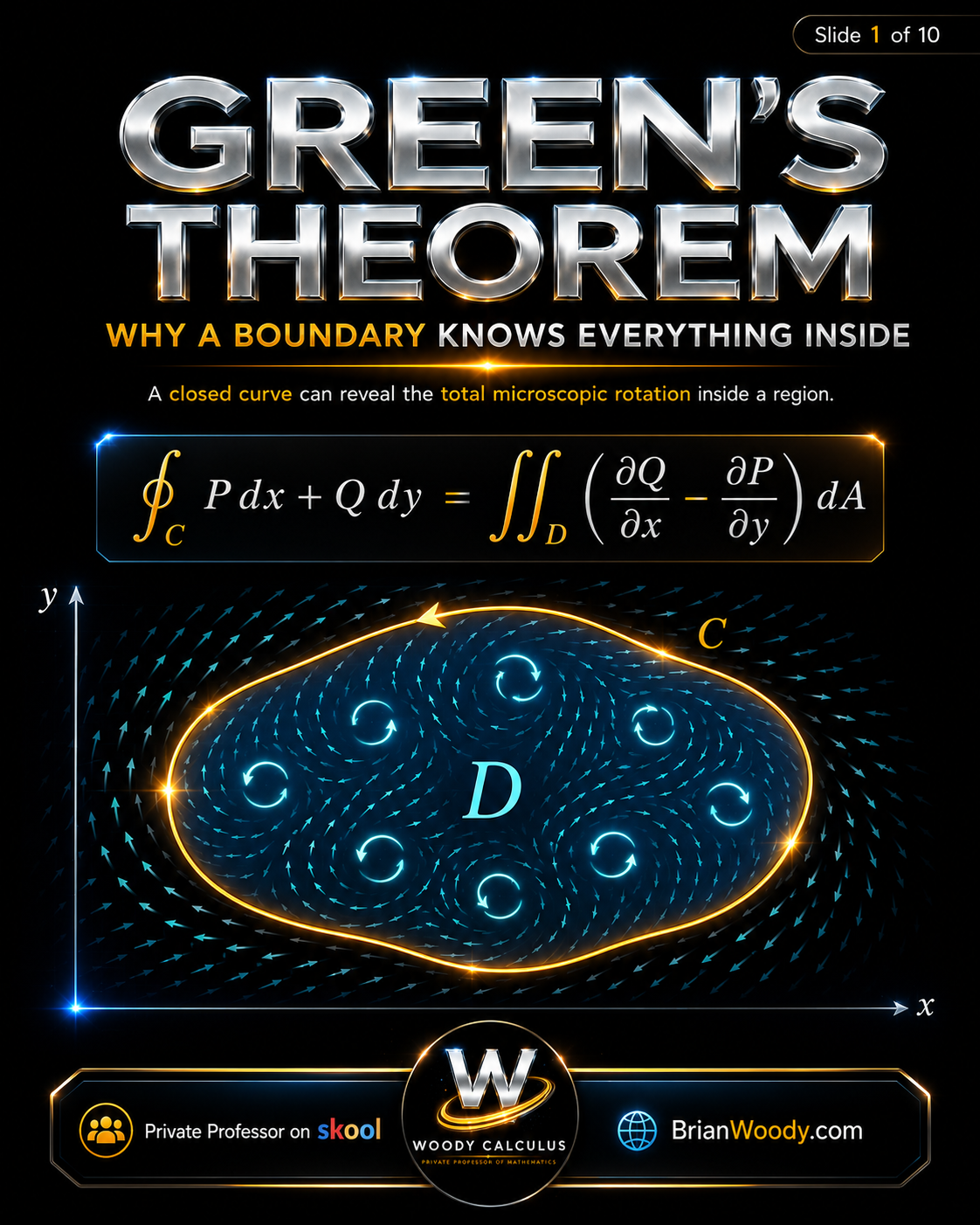
Green’s Theorem is one of the most important ideas in Calculus 3 and vector calculus. It says that a line integral around a closed boundary can reveal what is happening throughout the entire region inside that boundary.
At first, this can feel almost impossible. How can walking around the edge of a region tell you something about the total rotation inside the region?
That is the magic of the theorem.
In its circulation form:
\[
\oint_C P\,dx+Q\,dy
=
\iint_D
\left(
\frac{\partial Q}{\partial x}
–
\frac{\partial P}{\partial y}
\right)
\,dA.
\]
The left side is a boundary line integral. The right side is an interior double integral. The theorem says these two measurements are secretly the same.
Green’s Theorem Key Facts
- Green’s Theorem converts a closed line integral into a double integral over the region inside.
- The circulation form measures total curl or microscopic rotation inside a region.
- The curve \(C\) must be simple, closed, and positively oriented.
- Positive orientation means counterclockwise for an outer boundary.
- The region \(D\) is the interior enclosed by \(C\).
- The vector field is usually written \(F=\langle P,Q\rangle\).
- The 2D curl is \(\frac{\partial Q}{\partial x}-\frac{\partial P}{\partial y}\).
- This theorem is the two-dimensional bridge to Stokes’ Theorem and the Divergence Theorem.
This Woody Calculus visual lesson explains the idea in order: what the theorem says, what ingredients are required, how curl appears inside the region, how to compute a full worked example, how the boundary side agrees with the area side, how the flux form works, how to compute area from a boundary, and when to use the theorem on exams.
What Is Green’s Theorem?
Green’s Theorem is a result in vector calculus that connects a line integral around a closed curve to a double integral over the region inside the curve.
Suppose \(C\) is a positively oriented, simple, closed curve in the plane, and suppose \(D\) is the region enclosed by \(C\). If \(P\) and \(Q\) have continuous first partial derivatives on an open region containing \(D\), then:
\[
\oint_C P\,dx+Q\,dy
=
\iint_D
\left(
\frac{\partial Q}{\partial x}
–
\frac{\partial P}{\partial y}
\right)
\,dA.
\]
The expression
\[
\frac{\partial Q}{\partial x}
–
\frac{\partial P}{\partial y}
\]
is the two-dimensional curl of the vector field \(F=\langle P,Q\rangle\). It measures local rotation.
If you add up all the microscopic rotation inside \(D\), you get the total circulation around the boundary \(C\).
What Green’s Theorem Says
The core message is:
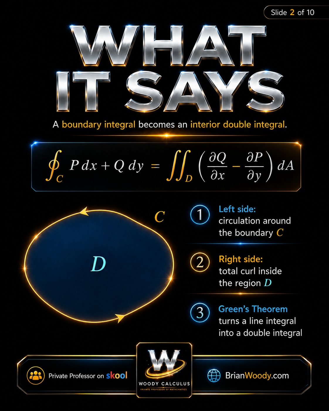
A boundary integral becomes an interior double integral.
The formula is:
\[
\oint_C P\,dx+Q\,dy
=
\iint_D
\left(
\frac{\partial Q}{\partial x}
–
\frac{\partial P}{\partial y}
\right)
\,dA.
\]
The left side,
\[
\oint_C P\,dx+Q\,dy,
\]
measures circulation around the boundary. It tells you how much the vector field pushes along the closed curve \(C\).
The right side,
\[
\iint_D
\left(
\frac{\partial Q}{\partial x}
–
\frac{\partial P}{\partial y}
\right)
\,dA,
\]
adds up the curl inside the region. It measures the total microscopic rotation over the entire region \(D\).
That means the theorem can turn a difficult line integral into a potentially easier double integral, or turn a difficult double integral into a potentially easier line integral.
That flexibility is why it is so powerful on exams.
The Ingredients of Green’s Theorem
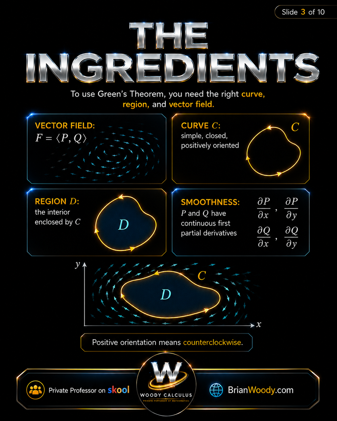
To use the theorem correctly, you need the right curve, region, and vector field.
The vector field is
\[
F=\langle P,Q\rangle.
\]
The curve \(C\) must be:
- simple, meaning it does not cross itself,
- closed, meaning it returns to its starting point,
- positively oriented, meaning counterclockwise for an outer boundary.
The region \(D\) is the interior enclosed by \(C\).
The functions \(P\) and \(Q\) must have continuous first partial derivatives on a region containing \(D\). In practice, students often check that \(P\), \(Q\), and their first partial derivatives are smooth on and inside the curve.
The most common student mistakes are:
- using the theorem on a curve that is not closed,
- forgetting the orientation,
- using the wrong curl order,
- forgetting that clockwise orientation changes the sign,
- ignoring holes or singularities inside the region.
The Curl Inside the Region
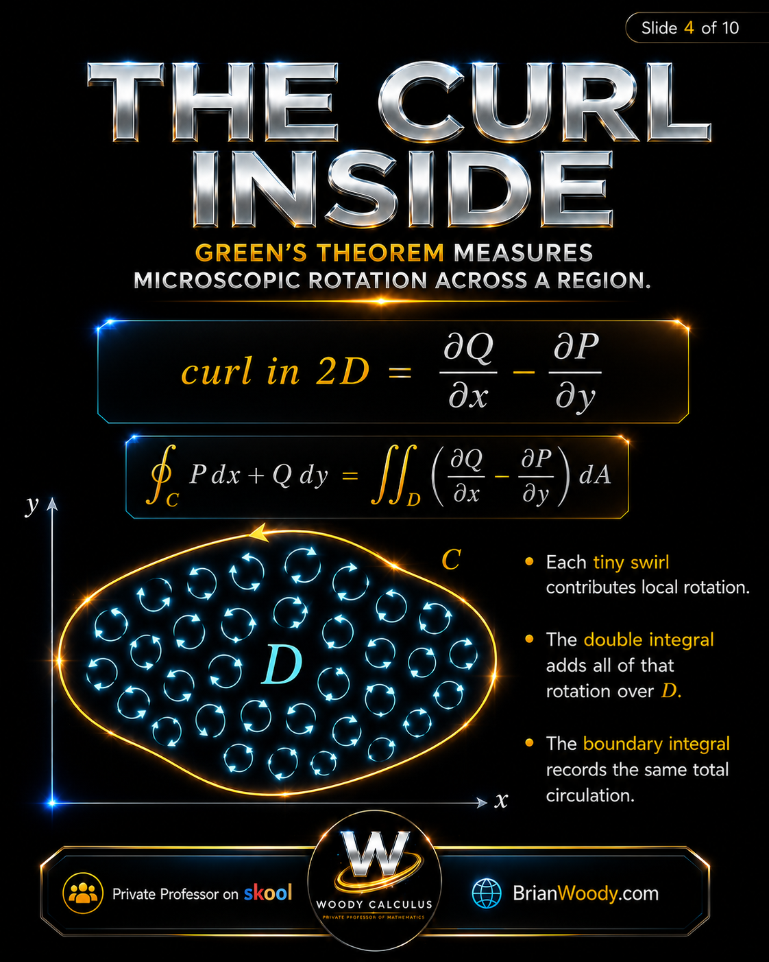
The circulation form measures microscopic rotation across a region.
For a two-dimensional vector field
\[
F=\langle P,Q\rangle,
\]
the scalar curl is:
\[
\operatorname{curl}_{2D}(F)
=
\frac{\partial Q}{\partial x}
–
\frac{\partial P}{\partial y}.
\]
This quantity measures how much the vector field tends to rotate around a tiny point.
Think of placing tiny paddle wheels throughout the vector field. If the field causes a small paddle wheel to spin counterclockwise, the curl is positive. If it spins clockwise, the curl is negative. If the paddle wheel does not spin, the curl is zero.
The boundary circulation equals the sum of all these tiny interior rotations:
\[
\oint_C P\,dx+Q\,dy
=
\iint_D \operatorname{curl}_{2D}(F)\,dA.
\]
This is the big conceptual leap:
The boundary records the total rotation inside.
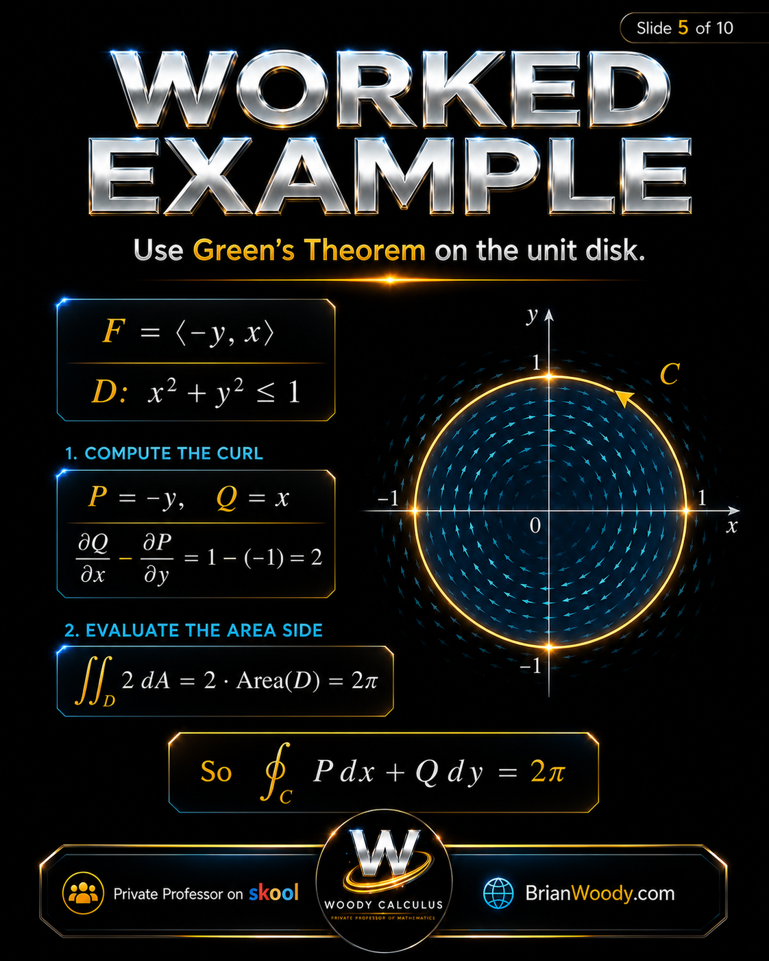
Worked Example: Green’s Theorem on the Unit Disk
Now let’s compute a full example.
Let
\[
F=\langle -y,x\rangle.
\]
So
\[
P=-y,
\qquad
Q=x.
\]
Let \(D\) be the unit disk:
\[
D:\ x^2+y^2\le 1.
\]
The boundary \(C\) is the unit circle, oriented counterclockwise.
We want to compute
\[
\oint_C P\,dx+Q\,dy.
\]
Using the theorem:
\[
\oint_C P\,dx+Q\,dy
=
\iint_D
\left(
\frac{\partial Q}{\partial x}
–
\frac{\partial P}{\partial y}
\right)
\,dA.
\]
Compute the curl:
\[
\frac{\partial Q}{\partial x}
=
\frac{\partial}{\partial x}(x)
=
1,
\]
and
\[
\frac{\partial P}{\partial y}
=
\frac{\partial}{\partial y}(-y)
=
-1.
\]
Therefore,
\[
\frac{\partial Q}{\partial x}
–
\frac{\partial P}{\partial y}
=
1-(-1)
=
2.
\]
So the line integral becomes:
\[
\oint_C P\,dx+Q\,dy
=
\iint_D 2\,dA.
\]
Since \(D\) is the unit disk, its area is \(\pi\). Therefore:
\[
\iint_D 2\,dA
=
2\operatorname{Area}(D)
=
2\pi.
\]
So:
\[
\oint_C P\,dx+Q\,dy=2\pi.
\]
The boundary circulation problem turned into a simple area calculation.
Boundary Side: Compute the Line Integral Directly
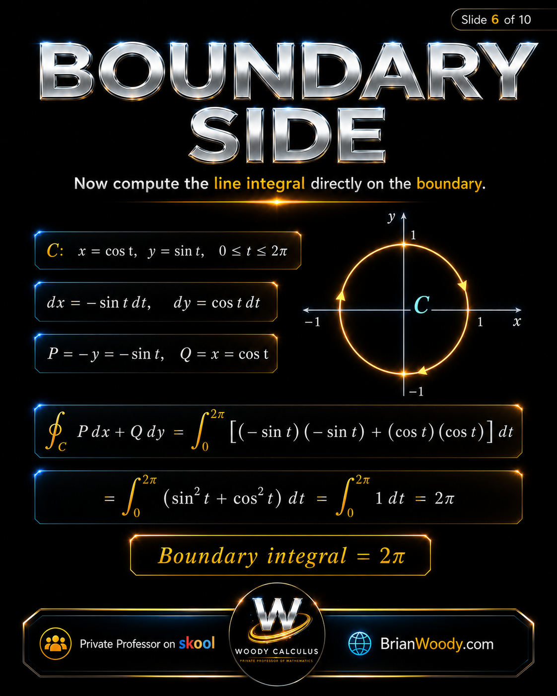
Now let’s verify the same answer by computing the boundary line integral directly.
The unit circle can be parametrized by:
\[
x=\cos t,
\qquad
y=\sin t,
\qquad
0\le t\le 2\pi.
\]
Then:
\[
dx=-\sin t\,dt,
\qquad
dy=\cos t\,dt.
\]
Since \(P=-y\) and \(Q=x\), along the curve:
\[
P=-\sin t,
\qquad
Q=\cos t.
\]
Now substitute into the line integral:
\[
\oint_C P\,dx+Q\,dy
=
\int_0^{2\pi}
\left[
(-\sin t)(-\sin t)
+
(\cos t)(\cos t)
\right]
\,dt.
\]
Simplify:
\[
\int_0^{2\pi}
(\sin^2 t+\cos^2 t)
\,dt
=
\int_0^{2\pi}1\,dt.
\]
Therefore:
\[
\oint_C P\,dx+Q\,dy=2\pi.
\]
This matches the interior-curl computation exactly.
That is the point: the boundary integral and the interior curl integral are two different ways of measuring the same total rotation.
Flux Form of Green’s Theorem
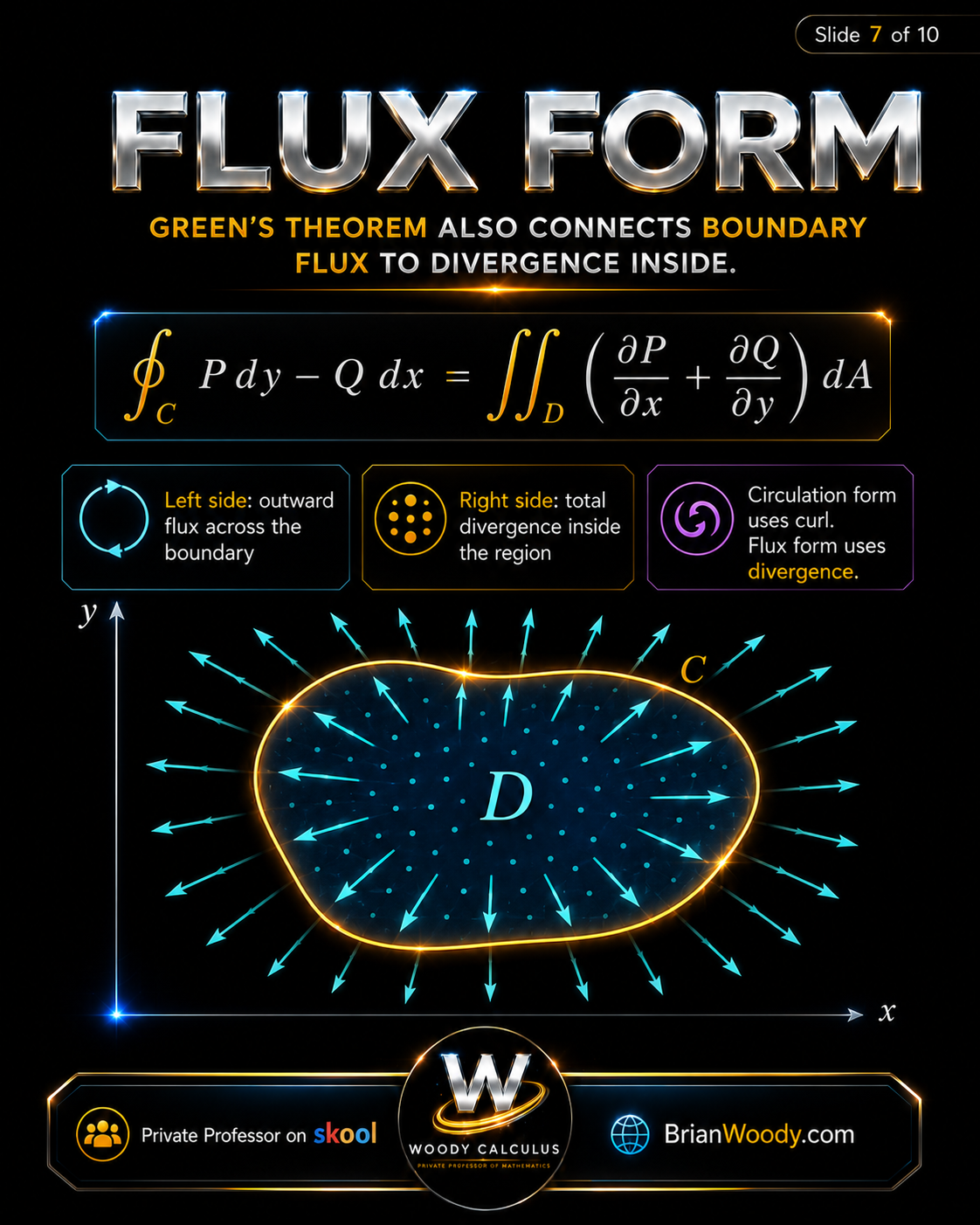
Green’s Theorem also has a flux form.
The circulation form uses curl:
\[
\oint_C P\,dx+Q\,dy
=
\iint_D
\left(
\frac{\partial Q}{\partial x}
–
\frac{\partial P}{\partial y}
\right)
\,dA.
\]
The flux form uses divergence:
\[
\oint_C P\,dy-Q\,dx
=
\iint_D
\left(
\frac{\partial P}{\partial x}
+
\frac{\partial Q}{\partial y}
\right)
\,dA.
\]
The left side represents outward flux across the boundary. The right side represents total divergence inside the region.
The divergence of \(F=\langle P,Q\rangle\) is:
\[
\nabla\cdot F
=
\frac{\partial P}{\partial x}
+
\frac{\partial Q}{\partial y}.
\]
So the flux form can be written as:
\[
\oint_C P\,dy-Q\,dx
=
\iint_D \nabla\cdot F\,dA.
\]
Circulation form asks: how much does the vector field swirl?
Flux form asks: how much does the vector field flow outward?
Both forms measure different physical behaviors.
Area from the Boundary
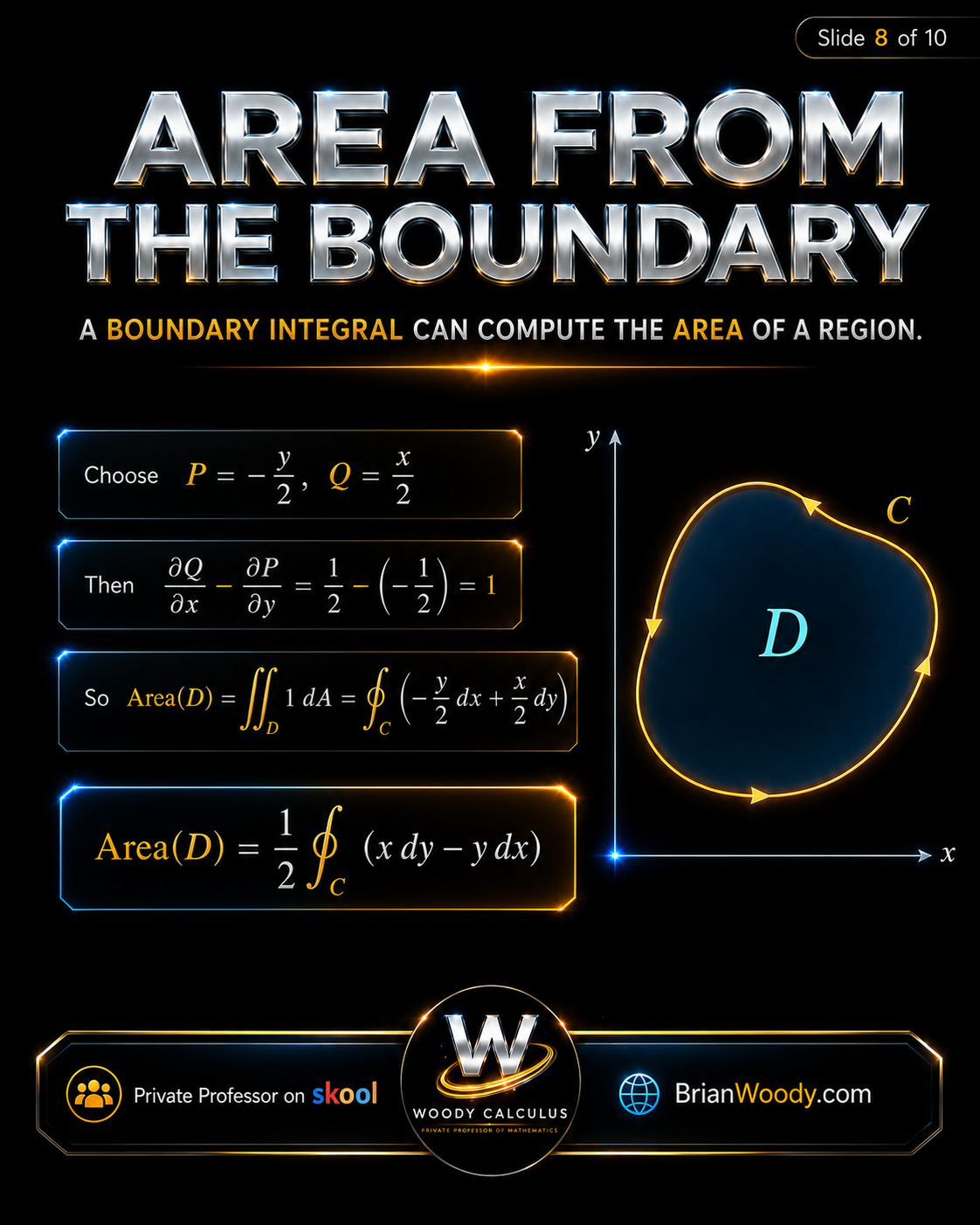
One of the most beautiful consequences is that a boundary integral can compute the area of a region.
We want the right side to become:
\[
\iint_D 1\,dA
=
\operatorname{Area}(D).
\]
To make that happen, choose
\[
P=-\frac{y}{2},
\qquad
Q=\frac{x}{2}.
\]
Then:
\[
\frac{\partial Q}{\partial x}
=
\frac{1}{2},
\qquad
\frac{\partial P}{\partial y}
=
-\frac{1}{2}.
\]
Therefore:
\[
\frac{\partial Q}{\partial x}
–
\frac{\partial P}{\partial y}
=
\frac{1}{2}-\left(-\frac{1}{2}\right)
=
1.
\]
By the theorem:
\[
\operatorname{Area}(D)
=
\iint_D 1\,dA
=
\oint_C
\left(
-\frac{y}{2}\,dx
+
\frac{x}{2}\,dy
\right).
\]
So:
\[
\operatorname{Area}(D)
=
\frac{1}{2}
\oint_C
(x\,dy-y\,dx).
\]
This formula is powerful because it computes area using only the boundary curve.
For a parametrized closed curve \(C: x=x(t), y=y(t)\), this becomes:
\[
\operatorname{Area}(D)
=
\frac{1}{2}
\int_a^b
\left(
x(t)y^{\prime}(t)-y(t)x^{\prime}(t)
\right)
\,dt.
\]
That is the boundary turning into area.
When to Use Green’s Theorem
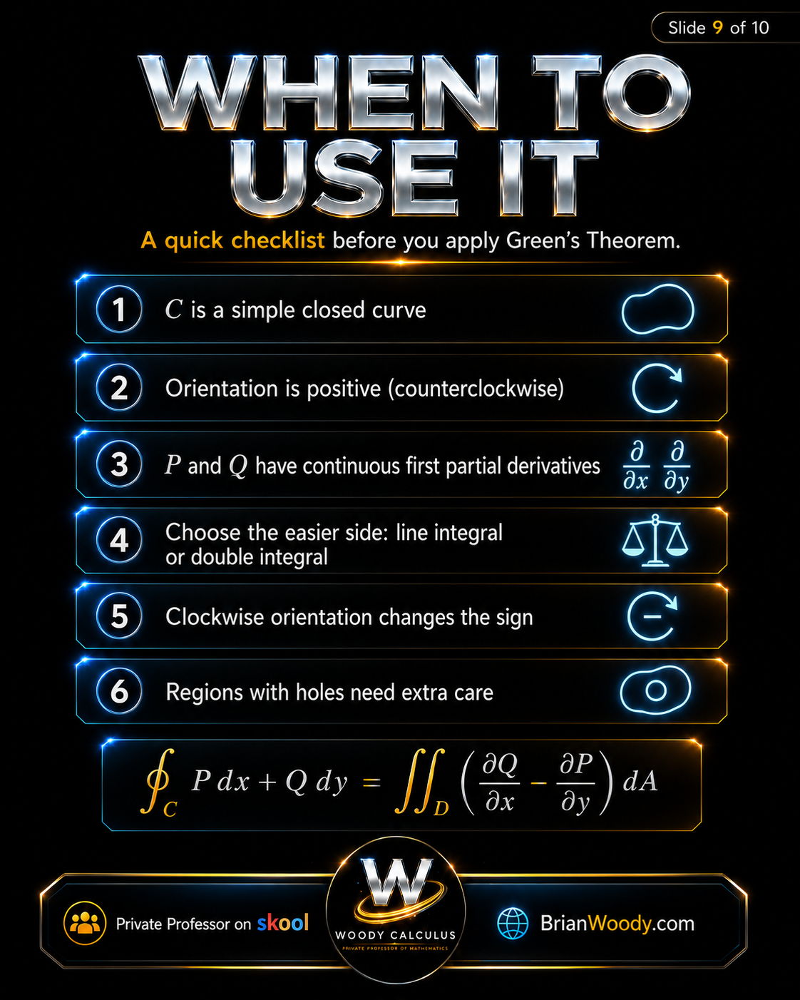
Before applying Green’s Theorem, use this checklist.
- Check that \(C\) is a simple closed curve.
- Check that the orientation is positive, meaning counterclockwise for the outer boundary.
- Check that \(P\) and \(Q\) have continuous first partial derivatives on and inside the region.
- Choose the easier side: line integral or double integral.
- Remember that clockwise orientation changes the sign.
- Be careful with holes, singularities, and regions that are not simply connected.
This theorem is especially useful when the boundary integral looks difficult but the curl is simple.
For example, if
\[
\frac{\partial Q}{\partial x}
–
\frac{\partial P}{\partial y}
\]
simplifies to a constant, then the double integral may collapse into a simple area calculation.
It is also useful in reverse. Sometimes the double integral is hard, but the boundary is easy to parametrize. Then you can replace the area integral with a line integral.
The decision is strategic:
Use whichever side is easier.
Important note about holes
If a region has a hole, the boundary has more than one component. The outer boundary is oriented counterclockwise, while inner boundaries are oriented clockwise for positive orientation of the region.
This is one of the most common places students lose signs.
How Green’s Theorem Connects to Stokes’ Theorem and the Divergence Theorem
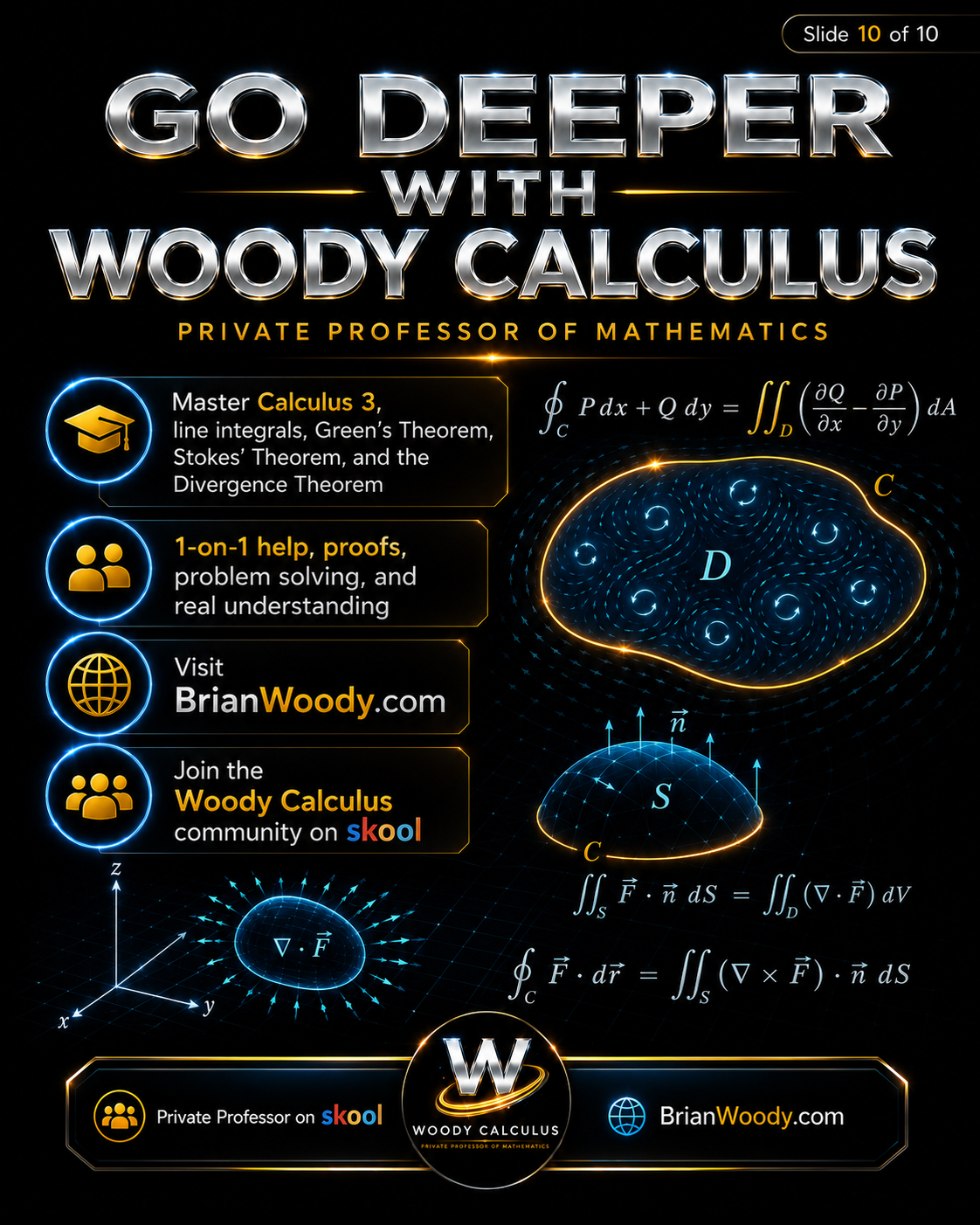
This is not an isolated trick. It is part of a larger family of theorems that connect boundaries to interiors.
The circulation form says:
\[
\oint_C P\,dx+Q\,dy
=
\iint_D
\left(
\frac{\partial Q}{\partial x}
–
\frac{\partial P}{\partial y}
\right)
\,dA.
\]
Stokes’ Theorem says:
\[
\oint_C \vec F\cdot d\vec r
=
\iint_S
(\nabla\times \vec F)\cdot \vec n\,dS.
\]
This is the three-dimensional version of the same idea: boundary circulation equals total curl through a surface.
The flux form says:
\[
\oint_C P\,dy-Q\,dx
=
\iint_D
\left(
\frac{\partial P}{\partial x}
+
\frac{\partial Q}{\partial y}
\right)
\,dA.
\]
The Divergence Theorem says:
\[
\iint_S \vec F\cdot \vec n\,dS
=
\iiint_E
\nabla\cdot \vec F\,dV.
\]
This is the three-dimensional version of boundary flux equals total divergence inside.
The deeper pattern is:
- Green’s Theorem connects a curve boundary to a planar region.
- Stokes’ Theorem connects a curve boundary to a surface.
- The Divergence Theorem connects a closed surface boundary to a solid region.
All of them express one central idea:
A boundary can know what happens inside.
More Green’s Theorem Examples
Example 1: A constant curl field over a rectangle
Let
\[
F=\langle -y,x\rangle,
\]
and let \(D\) be the rectangle \(0\le x\le 3\), \(0\le y\le 2\), with positively oriented boundary \(C\).
As before:
\[
P=-y,
\qquad
Q=x.
\]
The curl is:
\[
\frac{\partial Q}{\partial x}
–
\frac{\partial P}{\partial y}
=
1-(-1)
=
2.
\]
Therefore:
\[
\oint_C P\,dx+Q\,dy
=
\iint_D 2\,dA
=
2\operatorname{Area}(D).
\]
The rectangle has area \(3\cdot 2=6\), so:
\[
\oint_C P\,dx+Q\,dy=2(6)=12.
\]
The theorem avoided parametrizing all four sides of the rectangle.
Example 2: A gradient field with zero circulation
Let
\[
F=\langle 2x,2y\rangle.
\]
Then \(P=2x\) and \(Q=2y\). The curl is:
\[
\frac{\partial Q}{\partial x}
–
\frac{\partial P}{\partial y}
=
0-0
=
0.
\]
So for any simple closed curve \(C\) enclosing a region where the field is smooth:
\[
\oint_C 2x\,dx+2y\,dy
=
\iint_D 0\,dA
=
0.
\]
This makes sense because \(F=\nabla(x^2+y^2)\) is a gradient field. A gradient field has zero circulation around any closed curve contained in its domain.
Example 3: Area of an ellipse from its boundary
Consider the ellipse
\[
x=a\cos t,
\qquad
y=b\sin t,
\qquad
0\le t\le 2\pi.
\]
Using the boundary area formula:
\[
\operatorname{Area}(D)
=
\frac{1}{2}
\int_0^{2\pi}
\left(
x(t)y^{\prime}(t)-y(t)x^{\prime}(t)
\right)
\,dt.
\]
Compute:
\[
x(t)=a\cos t,
\qquad
y^{\prime}(t)=b\cos t,
\]
and
\[
y(t)=b\sin t,
\qquad
x^{\prime}(t)=-a\sin t.
\]
Therefore:
\[
x(t)y^{\prime}(t)-y(t)x^{\prime}(t)
=
ab\cos^2 t+ab\sin^2 t
=
ab.
\]
So:
\[
\operatorname{Area}(D)
=
\frac{1}{2}
\int_0^{2\pi}
ab\,dt
=
\frac{1}{2}(2\pi ab)
=
\pi ab.
\]
This gives the standard area formula for an ellipse.
Key Takeaways
- Green’s Theorem converts a closed line integral into a double integral over the enclosed region.
- The circulation form uses curl: \(\frac{\partial Q}{\partial x}-\frac{\partial P}{\partial y}\).
- The flux form uses divergence: \(\frac{\partial P}{\partial x}+\frac{\partial Q}{\partial y}\).
- Positive orientation means counterclockwise for an outer boundary.
- Clockwise orientation changes the sign of the line integral.
- This theorem can make difficult boundary integrals much easier.
- It can compute area from a boundary integral.
- It is the two-dimensional foundation for Stokes’ Theorem and the Divergence Theorem.
Green’s Theorem FAQ
What is Green’s Theorem?
Green’s Theorem is a vector calculus theorem that converts a line integral around a positively oriented closed curve into a double integral over the region inside the curve.
What is the formula for Green’s Theorem?
The circulation form is \(\oint_C P\,dx+Q\,dy=\iint_D(\partial Q/\partial x-\partial P/\partial y)\,dA\), where \(C\) is the positively oriented boundary of \(D\).
What does Green’s Theorem mean conceptually?
Conceptually, total circulation around a boundary equals the total curl inside the region. The boundary records the accumulated microscopic rotation in the interior.
What is positive orientation in Green’s Theorem?
For a simple closed outer boundary, positive orientation means counterclockwise. If the curve is oriented clockwise, the line integral changes sign.
What is the difference between circulation form and flux form?
The circulation form measures curl and uses \(\oint_C P\,dx+Q\,dy\). The flux form measures divergence and uses \(\oint_C P\,dy-Q\,dx\).
Can Green’s Theorem be used to find area?
Yes. Choosing \(P=-y/2\) and \(Q=x/2\) gives \(\operatorname{Area}(D)=\frac12\oint_C(x\,dy-y\,dx)\).
How is Green’s Theorem related to Stokes’ Theorem?
Green’s Theorem is a two-dimensional version of Stokes’ Theorem. Both connect boundary circulation to interior curl.
Master Green’s Theorem in Calculus 3
This theorem is not just a formula. It is one of the main bridges between line integrals, double integrals, vector fields, curl, flux, Stokes’ Theorem, and the Divergence Theorem.
To master it, students need to connect:
- Line integrals: circulation around a boundary.
- Double integrals: total curl or divergence inside a region.
- Orientation: counterclockwise versus clockwise signs.
- Curl: microscopic rotation.
- Flux: outward flow across a boundary.
- Area: boundary integrals can compute interior area.
- Stokes and Divergence: Green’s Theorem is the 2D gateway to the major theorems of vector calculus.
At Woody Calculus, students build fluency through clean setup, repeated perfect solutions, formula memorization, pattern recognition, and saying every step out loud until the process becomes automatic.
Green’s Theorem is the moment a boundary starts speaking for the entire region inside.
— Brian M. Woody
If you are studying Calculus 3, vector fields, line integrals, double integrals, Stokes’ Theorem, the Divergence Theorem, or advanced mathematics, this is one of the ideas you want to understand deeply.
Join Woody Calculus Mastery Lab on Skool
Related Woody Calculus Mathematical Essays
Explore more Woody Calculus visual lessons and deep-dive mathematical essays connecting
Calculus 3,
Calculus 2,
Differential Equations,
Linear Algebra,
Abstract Algebra,
Real Analysis,
Jacobians,
determinants,
and peak performance study methods and advanced problem-solving.
- How to Learn Calculus and Advanced Mathematics: A Peak Performance Study Guide
- Line Integrals and Vector Fields: What They Measure in Calculus 3
- The Jacobian Explained: The Hidden Scale Factor in Calculus III
- The Determinant Explained: The Number That Measures How a Matrix Changes Space
- Eigenvalues and Eigenvectors Explained: The Special Directions That Unlock Linear Algebra
- Laplace Transforms Explained: Turning Differential Equations Into Algebra
- Fourier Series Explained: Harmonics, Sound, Heat, and Quantum Mechanics
- Möbius Strip Explained: Orientation, Vector Calculus, and Stokes’ Theorem
- View All Woody Calculus Blog Posts
Related University Math Help Pages
Woody Calculus supports students at major universities with structured help in Calculus III, Differential Equations, Linear Algebra, Calculus II, Abstract Algebra, Real Analysis, and advanced mathematics. For a full list of supported schools, visit the University Calculus Tutor Hub.
- University Calculus Tutor Hub
- Purdue University Calculus Tutor
- University of Florida Calculus Tutor
- Colorado State University Calculus Help
- UCF Calculus Tutor
- Auburn University Calculus Tutor
- University of Nevada, Reno Calculus Tutor
Trusted by Students Nationwide
The Woody Calculus Mastery Lab gives university students access to structured mathematics support, written solutions, video lessons, exam-focused training, and expert guidance from Brian M. Woody.
Students use Woody Calculus for Calculus III, Differential Equations, Linear Algebra, Calculus II, Abstract Algebra, Real Analysis, and other advanced mathematics courses.