Stokes’ Theorem is one of the most powerful ideas in Calculus 3 and vector calculus. It says that the circulation around the edge of a surface equals the total curl passing through the surface.
In other words:
The edge knows the surface.
Students often search for Stokes theorem Calculus 3 help because this topic brings together line integrals, surface integrals, curl, normals, orientation, and the right-hand rule all at once.
The theorem connects a line integral around a boundary curve to a surface integral of curl:
\[
\oint_C \vec F\cdot d\vec r
=
\iint_S
(\nabla\times \vec F)\cdot \vec n\,dS.
\]
The left side measures boundary circulation. The right side adds up the curl through the surface. Stokes’ Theorem says these two measurements are the same when the surface and boundary are oriented correctly.
Estimated read time: 12 minutes.
Quick summary: Stokes’ Theorem converts a boundary line integral into a surface integral of curl. Use it when one side is easier to compute than the other. The key checks are: \(C\) is closed, \(C=\partial S\), the orientation matches the right-hand rule, and the vector field is smooth on the required surface.
Stokes’ Theorem Key Facts
- Stokes’ Theorem converts a line integral around a closed curve into a surface integral of curl.
- The boundary curve \(C\) must be the boundary of the surface: \(C=\partial S\).
- The surface \(S\) must be oriented with a compatible unit normal vector \(\vec n\).
- The positive boundary direction is determined by the right-hand rule.
- The curl \(\nabla\times \vec F\) measures local rotation of the vector field.
- Reverse the orientation, and the integral changes sign.
- Different surfaces with the same oriented boundary give the same value when the vector field is smooth on the relevant region.
- Green’s Theorem is the flat two-dimensional case of Stokes’ Theorem.
From Woody Calculus Instagram to Full Lesson
This article expands a Woody Calculus Instagram carousel into a complete online lesson on Stokes’ Theorem, with definitions, formulas, worked examples, orientation checks, surface-integral strategy, boundary-integral verification, and related Calculus 3 links.
Follow @WoodyCalculus on Instagram for visual mathematics lessons, then use this page as the deeper study guide.
This Woody Calculus visual lesson explains Stokes’ Theorem in order: what the theorem says, what ingredients are required, how curl appears inside the surface, why orientation matters, why the same boundary can give the same answer for different spanning surfaces, how to compute a full worked example, how to verify the boundary side directly, and how Stokes’ Theorem connects to Green’s Theorem and the larger structure of vector calculus.
What Is Stokes’ Theorem?
Stokes’ Theorem is a vector calculus theorem that relates circulation around a closed boundary curve to curl through a surface.
Let \(S\) be a smooth oriented surface with boundary curve \(C=\partial S\). Let \(\vec F\) be a vector field with continuous partial derivatives on an open region containing \(S\). If the orientation of \(C\) is compatible with the chosen normal vector \(\vec n\), then:
\[
\oint_C \vec F\cdot d\vec r
=
\iint_S
(\nabla\times \vec F)\cdot \vec n\,dS.
\]
The left side,
\[
\oint_C \vec F\cdot d\vec r,
\]
is a line integral measuring circulation around the edge \(C\).
The right side,
\[
\iint_S
(\nabla\times \vec F)\cdot \vec n\,dS,
\]
is a surface integral measuring the total curl through the surface \(S\).
The theorem says that boundary circulation equals surface curl.
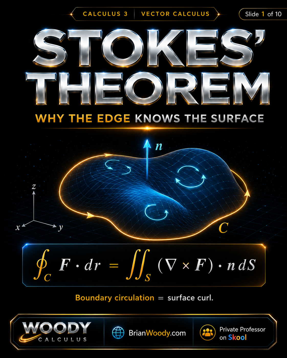
What Stokes’ Theorem Says
The core message is simple:
Walk the edge. Add the curl through the surface.
The formula is:
\[
\oint_C \vec F\cdot d\vec r
=
\iint_S
(\nabla\times \vec F)\cdot \vec n\,dS.
\]
The boundary curve \(C\) is the edge of the surface:
\[
C=\partial S.
\]
The line integral around \(C\) measures how strongly the vector field circulates along the boundary. The surface integral measures how much curl pierces the surface.
Stokes’ Theorem says those two measurements agree.
This is why the theorem is so useful in Calculus 3. Sometimes the boundary line integral is hard, but the surface integral is easy. Other times the surface integral looks difficult, but the boundary is easy to parameterize.
Use whichever side is easier.
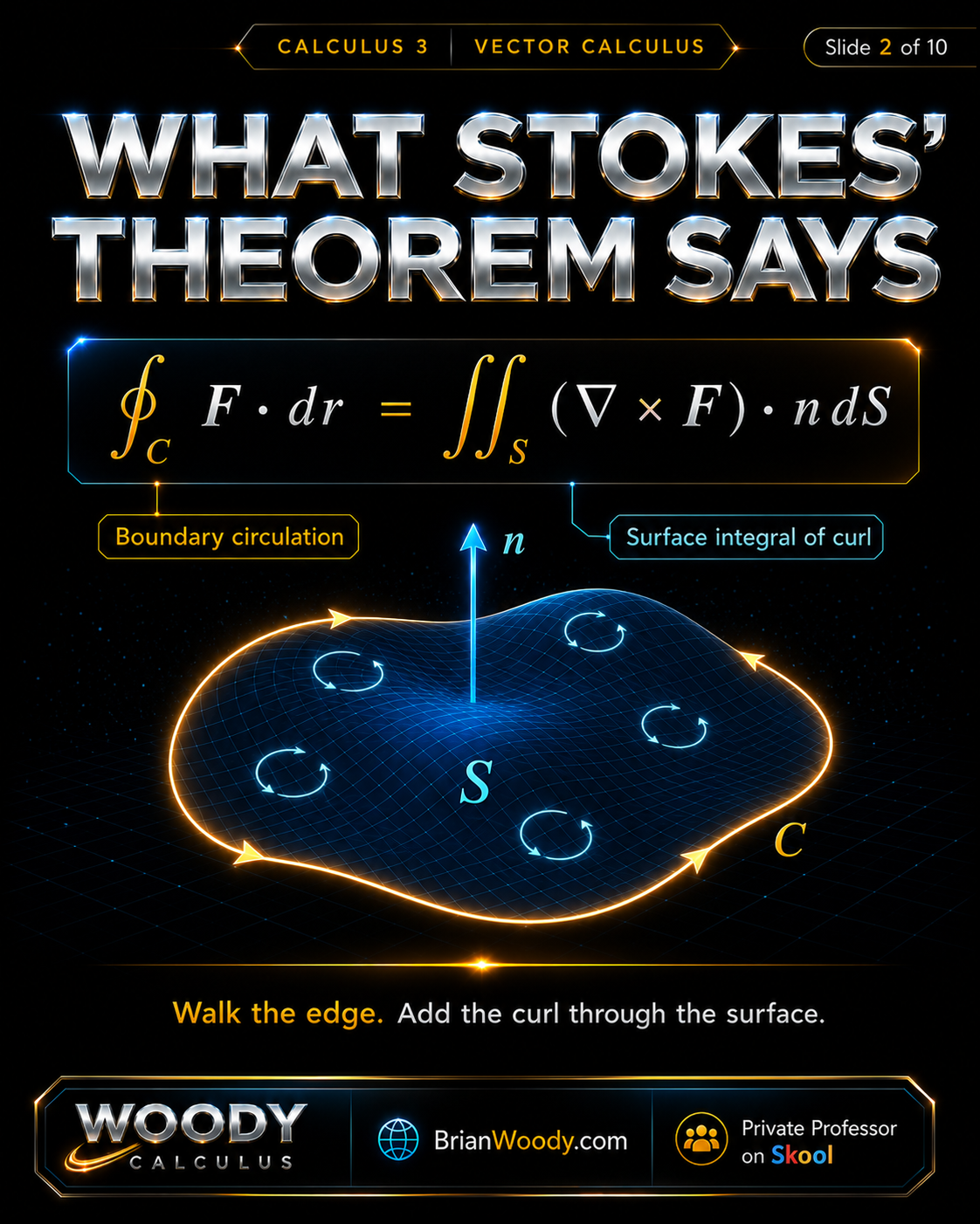
The Ingredients of Stokes’ Theorem
To use Stokes’ Theorem correctly, you need four ingredients.
- A vector field \(\vec F\).
- A smooth oriented surface \(S\).
- A closed boundary curve \(C=\partial S\).
- A compatible orientation determined by the right-hand rule.
The surface \(S\) must have a boundary curve \(C\). That means \(C\) is the edge of the surface.
The surface also needs an orientation. This is usually given by choosing a unit normal vector \(\vec n\).
Once you choose \(\vec n\), the positive direction around the boundary \(C\) is determined by the right-hand rule.
This orientation condition is not optional. If the boundary direction and normal vector do not match, the sign of the answer will be wrong.
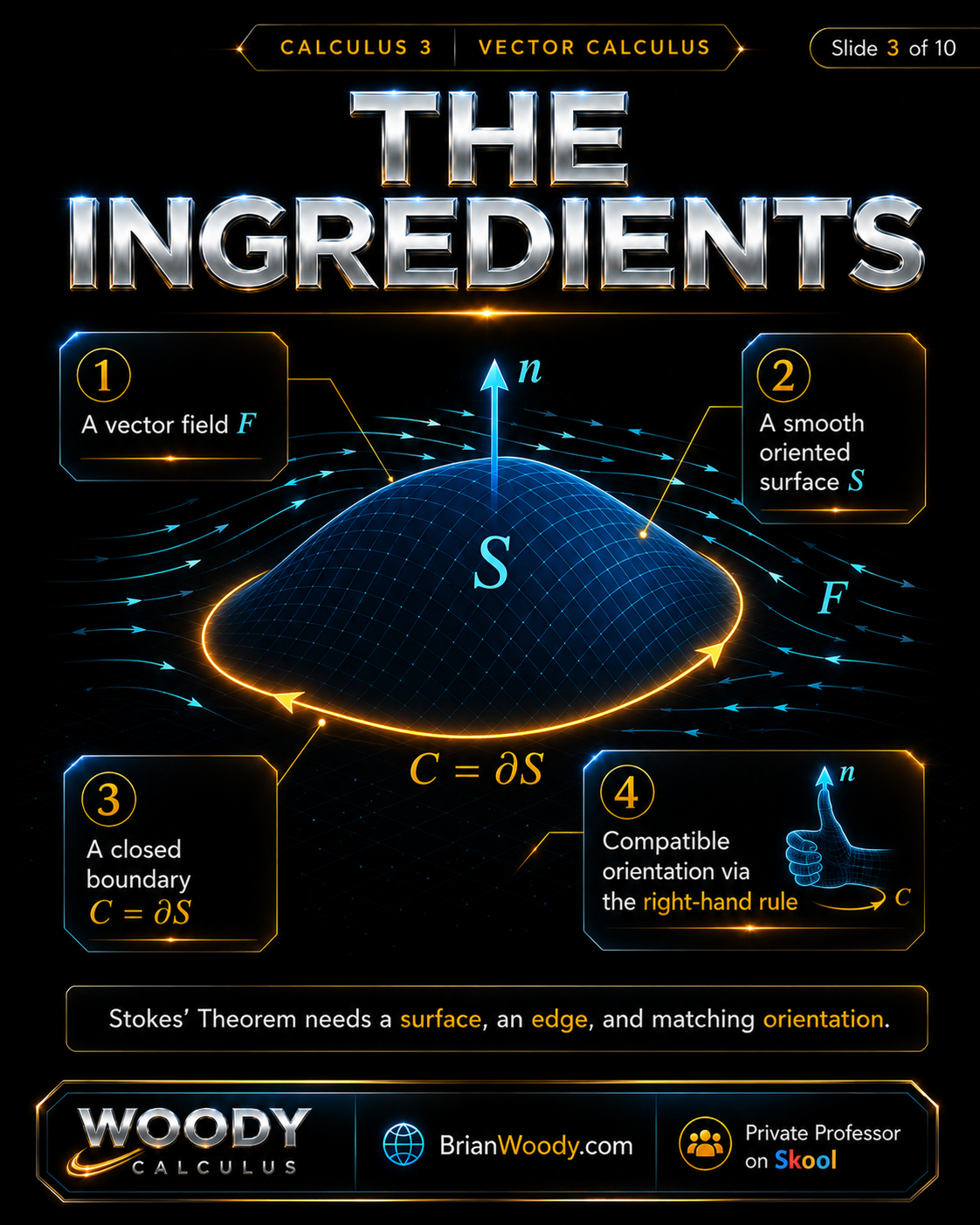
The Curl Inside Stokes’ Theorem
The surface side of Stokes’ Theorem uses curl.
For a vector field
\[
\vec F=\langle P,Q,R\rangle,
\]
the curl is:
\[
\nabla\times \vec F
=
\left\langle
\frac{\partial R}{\partial y}-\frac{\partial Q}{\partial z},
\frac{\partial P}{\partial z}-\frac{\partial R}{\partial x},
\frac{\partial Q}{\partial x}-\frac{\partial P}{\partial y}
\right\rangle.
\]
Curl measures local rotation in a vector field.
The dot product
\[
(\nabla\times \vec F)\cdot \vec n
\]
measures the component of curl passing through the surface in the chosen normal direction.
Then the surface integral
\[
\iint_S
(\nabla\times \vec F)\cdot \vec n\,dS
\]
adds that rotational contribution over the entire surface.
That is why Stokes’ Theorem can be understood as:
Total boundary circulation equals total surface rotation.
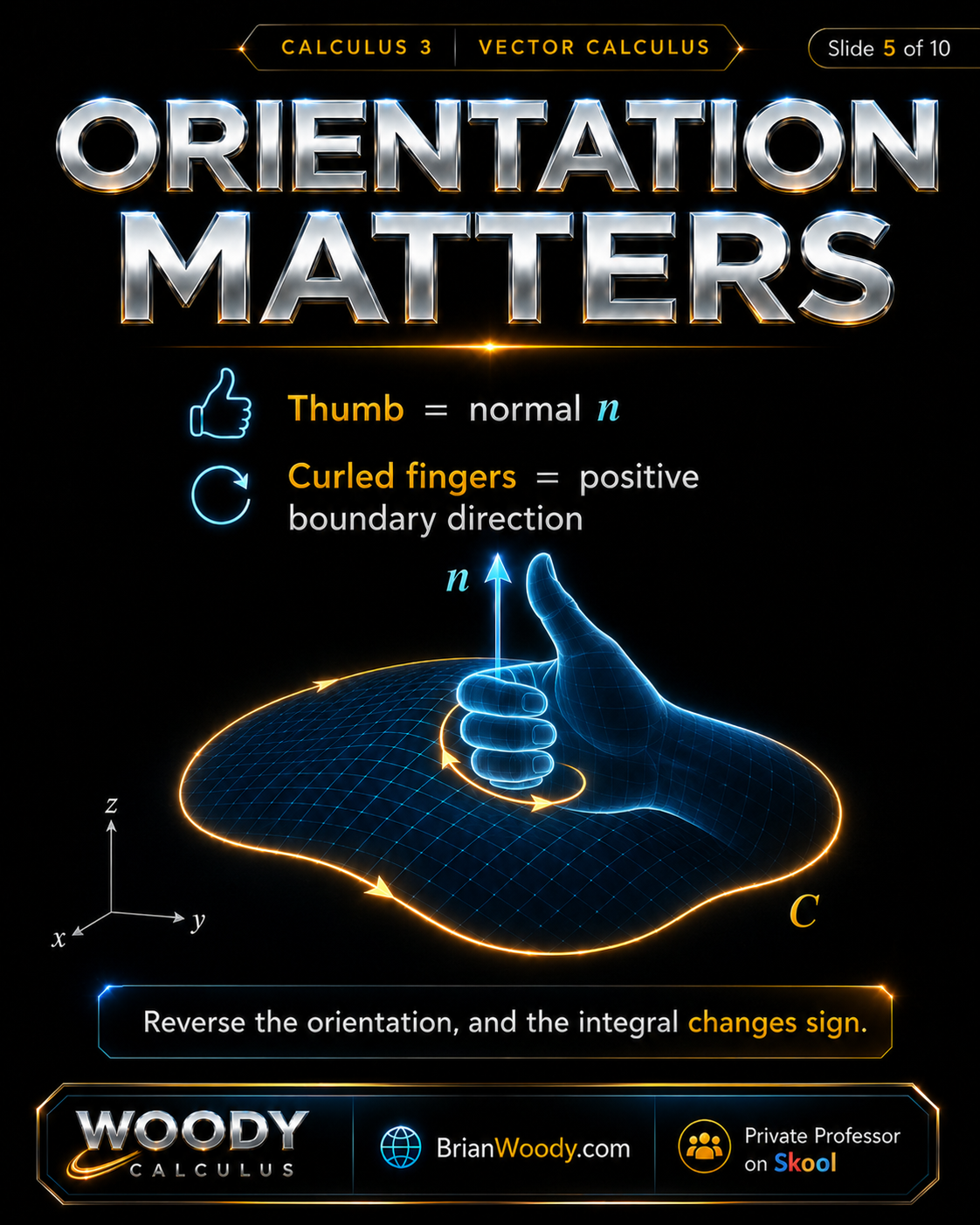
Why Orientation Matters
Orientation is one of the most important details in Stokes’ Theorem.
The rule is:
- Your thumb points in the direction of the chosen normal vector \(\vec n\).
- Your curled fingers point in the positive boundary direction around \(C\).
This is the right-hand rule.
If the normal vector points upward, the positive direction around a flat disk in the \(xy\)-plane is counterclockwise when viewed from above.
If you reverse the normal vector, the positive boundary direction reverses too.
That means:
Reverse the orientation, and the integral changes sign.
So before computing anything, always check whether the surface normal and boundary direction are compatible.
Same Edge, Same Answer
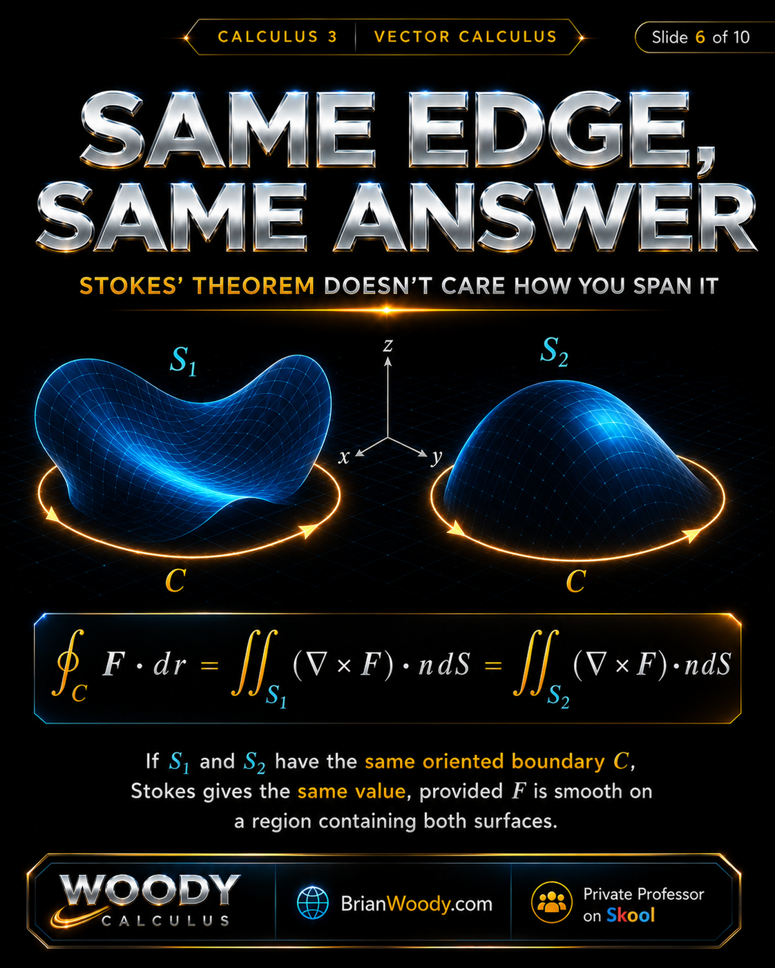
One of the most beautiful consequences of Stokes’ Theorem is that the answer depends on the oriented boundary, not on the particular surface you choose.
Suppose \(S_1\) and \(S_2\) are two oriented surfaces with the same oriented boundary \(C\). If \(\vec F\) is smooth on a region containing the surfaces, then:
\[
\oint_C \vec F\cdot d\vec r
=
\iint_{S_1}
(\nabla\times \vec F)\cdot \vec n\,dS
=
\iint_{S_2}
(\nabla\times \vec F)\cdot \vec n\,dS.
\]
This means you can often choose the easier surface.
For example, if \(C\) is a circle in space, one surface spanning \(C\) might be curved and complicated, while another might be a flat disk. If the orientations match and the vector field is smooth, Stokes’ Theorem allows you to use the easier surface.
Same edge. Same circulation. Same answer.
Worked Example: Stokes’ Theorem on the Unit Disk
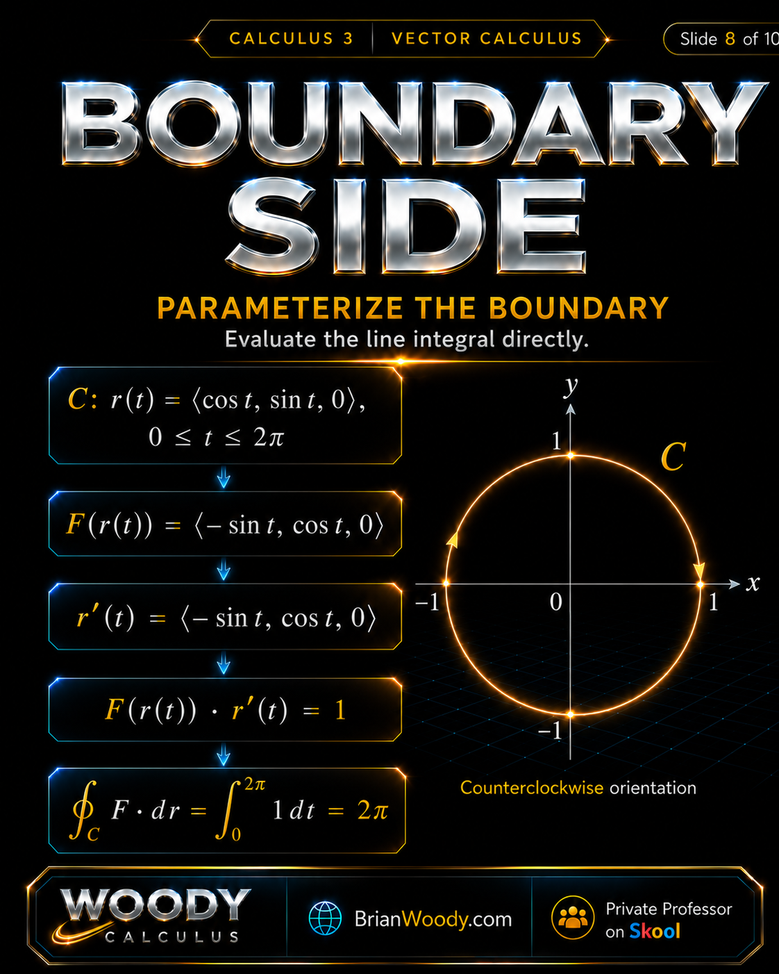
Now let’s compute a full example.
Let
\[
\vec F=\langle -y,x,0\rangle.
\]
Let \(S\) be the unit disk in the plane \(z=0\):
\[
x^2+y^2\le 1,
\qquad
z=0.
\]
Choose the upward unit normal:
\[
\vec n=\langle 0,0,1\rangle.
\]
The boundary \(C=\partial S\) is the unit circle oriented counterclockwise when viewed from above.
First compute the curl:
\[
\nabla\times \vec F
=
\nabla\times \langle -y,x,0\rangle.
\]
Here \(P=-y\), \(Q=x\), and \(R=0\). Therefore:
\[
\nabla\times \vec F
=
\langle 0,0,2\rangle.
\]
Now compute the surface integral:
\[
\iint_S
(\nabla\times \vec F)\cdot \vec n\,dS
=
\iint_S
\langle 0,0,2\rangle\cdot \langle 0,0,1\rangle\,dS.
\]
The dot product is:
\[
\langle 0,0,2\rangle\cdot \langle 0,0,1\rangle=2.
\]
So:
\[
\iint_S
(\nabla\times \vec F)\cdot \vec n\,dS
=
\iint_D 2\,dA.
\]
The disk has area \(\pi\), so:
\[
\iint_D 2\,dA=2\pi.
\]
By Stokes’ Theorem:
\[
\oint_C \vec F\cdot d\vec r=2\pi.
\]
Boundary Side: Compute the Line Integral Directly
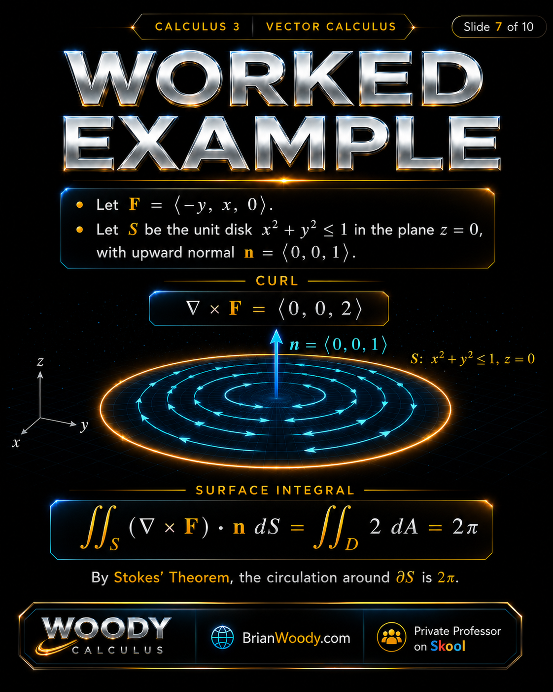
Now let’s verify the same answer from the boundary side.
The boundary curve is the unit circle:
\[
\vec r(t)=\langle \cos t,\sin t,0\rangle,
\qquad
0\le t\le 2\pi.
\]
Then:
\[
\vec r\, ‘(t)=\langle -\sin t,\cos t,0\rangle.
\]
Substitute the curve into the vector field:
\[
\vec F(\vec r(t))
=
\langle -\sin t,\cos t,0\rangle.
\]
Now compute the dot product:
\[
\vec F(\vec r(t))\cdot \vec r\, ‘(t)
=
\langle -\sin t,\cos t,0\rangle
\cdot
\langle -\sin t,\cos t,0\rangle.
\]
So:
\[
\vec F(\vec r(t))\cdot \vec r\, ‘(t)
=
\sin^2 t+\cos^2 t
=
1.
\]
Therefore:
\[
\oint_C \vec F\cdot d\vec r
=
\int_0^{2\pi}1\,dt
=
2\pi.
\]
This matches the surface integral exactly.
The boundary calculation and the surface-curl calculation give the same answer because they are two views of the same circulation.
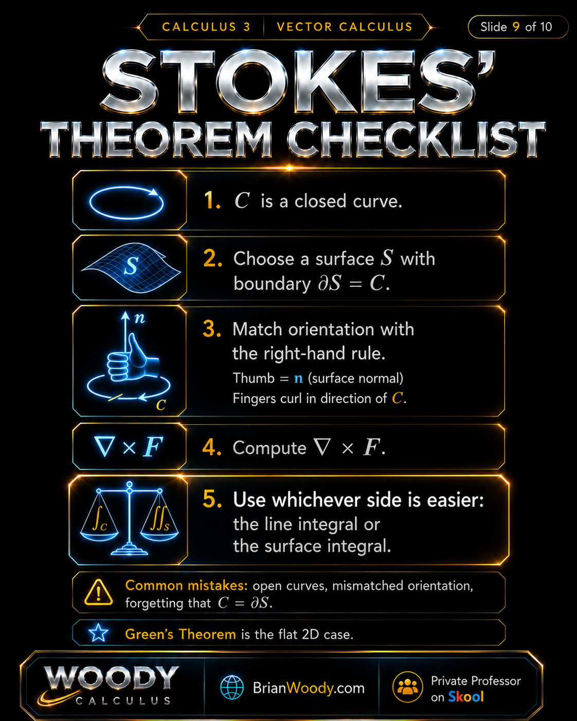
Stokes’ Theorem Checklist
Before applying Stokes’ Theorem, use this checklist.
- Check that \(C\) is a closed curve.
- Choose a surface \(S\) with boundary \(\partial S=C\).
- Match the orientation with the right-hand rule.
- Compute the curl \(\nabla\times \vec F\).
- Use whichever side is easier: the line integral or the surface integral.
Common mistakes include:
- using an open curve,
- forgetting that \(C=\partial S\),
- using the wrong boundary direction,
- choosing a normal vector that does not match the boundary orientation,
- forgetting that reversing orientation changes the sign,
- using Stokes’ Theorem where the vector field is not smooth on the required region.
A good exam strategy is to ask:
Which side is easier?
If the boundary is easy to parameterize, compute the line integral. If the curl and surface are simple, use the surface integral.
How Stokes’ Theorem Connects to Green’s Theorem and the Divergence Theorem
Stokes’ Theorem is not just another vector calculus formula. It is part of a larger boundary-versus-interior pattern.
Green’s Theorem says:
\[
\oint_C P\,dx+Q\,dy
=
\iint_D
\left(
\frac{\partial Q}{\partial x}
–
\frac{\partial P}{\partial y}
\right)
\,dA.
\]
Stokes’ Theorem says:
\[
\oint_C \vec F\cdot d\vec r
=
\iint_S
(\nabla\times \vec F)\cdot \vec n\,dS.
\]
If the surface \(S\) is a flat region \(D\) in the \(xy\)-plane and \(\vec F=\langle P,Q,0\rangle\), then:
\[
(\nabla\times \vec F)\cdot \vec k
=
\frac{\partial Q}{\partial x}
–
\frac{\partial P}{\partial y}.
\]
So Green’s Theorem is the flat two-dimensional case of Stokes’ Theorem.
The Divergence Theorem is another member of the same family:
\[
\iint_S \vec F\cdot \vec n\,dS
=
\iiint_E
\nabla\cdot \vec F\,dV.
\]
The larger pattern is:
- Green’s Theorem connects a boundary curve to a flat region.
- Stokes’ Theorem connects a boundary curve to a surface.
- The Divergence Theorem connects a closed surface to a solid region.
All of them express the same deep idea:
A boundary can reveal what happens inside.

More Stokes’ Theorem Examples
Example 1: A circle of radius 2 in a horizontal plane
Let
\[
\vec F=\langle -y,x,0\rangle.
\]
Let \(C\) be the circle \(x^2+y^2=4\) in the plane \(z=3\), oriented counterclockwise when viewed from above.
Instead of parameterizing the circle, use the flat disk \(S\) inside it with upward normal:
\[
\vec n=\langle 0,0,1\rangle.
\]
As before:
\[
\nabla\times \vec F=\langle 0,0,2\rangle.
\]
So:
\[
(\nabla\times \vec F)\cdot \vec n=2.
\]
The disk has radius \(2\), so its area is \(4\pi\). Therefore:
\[
\oint_C \vec F\cdot d\vec r
=
\iint_S 2\,dS
=
2(4\pi)
=
8\pi.
\]
Stokes’ Theorem turns the line integral into a simple area calculation.
Example 2: A triangular surface in a plane
Let
\[
\vec F=\langle z,x,y\rangle.
\]
Let \(S\) be the triangle in the plane \(x+y+z=1\) in the first octant, oriented with normal vector pointing in the direction \(\langle 1,1,1\rangle\).
First compute the curl:
\[
\nabla\times \vec F
=
\left\langle
\frac{\partial y}{\partial y}-\frac{\partial x}{\partial z},
\frac{\partial z}{\partial z}-\frac{\partial y}{\partial x},
\frac{\partial x}{\partial x}-\frac{\partial z}{\partial y}
\right\rangle.
\]
So:
\[
\nabla\times \vec F=\langle 1,1,1\rangle.
\]
The unit normal is:
\[
\vec n=\frac{1}{\sqrt 3}\langle 1,1,1\rangle.
\]
Thus:
\[
(\nabla\times \vec F)\cdot \vec n
=
\langle 1,1,1\rangle\cdot
\frac{1}{\sqrt 3}\langle 1,1,1\rangle
=
\sqrt 3.
\]
The triangle has vertices \((1,0,0)\), \((0,1,0)\), and \((0,0,1)\). Each side has length \(\sqrt 2\), so the triangle is equilateral with area:
\[
\frac{\sqrt 3}{2}.
\]
Therefore:
\[
\oint_C \vec F\cdot d\vec r
=
\iint_S \sqrt 3\,dS
=
\sqrt 3\cdot \frac{\sqrt 3}{2}
=
\frac{3}{2}.
\]
So the circulation around the positively oriented boundary is:
\[
\frac{3}{2}.
\]
Example 3: Using a different surface with the same boundary
Let \(C\) be the unit circle in the \(xy\)-plane, oriented counterclockwise when viewed from above, and let:
\[
\vec F=\langle -y,x,0\rangle.
\]
Instead of using the flat disk, we could use the upper hemisphere:
\[
x^2+y^2+z^2=1,
\qquad z\ge 0,
\]
with the compatible orientation that induces the same positive boundary direction on \(C\).
This curved surface has the same boundary \(C\). Since the vector field is smooth, Stokes’ Theorem gives the same boundary circulation as the flat disk:
\[
\oint_C \vec F\cdot d\vec r=2\pi.
\]
This is the power of the theorem: choose the surface that makes the computation easiest.
Common Mistakes with Stokes’ Theorem
Stokes’ Theorem is conceptually beautiful, but students often lose points on setup.
Mistake 1: Forgetting that \(C=\partial S\)
The boundary curve must actually be the edge of the surface. If the surface does not have boundary \(C\), the theorem does not apply.
Mistake 2: Mismatching orientation
The surface normal and boundary direction must match by the right-hand rule. If they do not match, the answer changes sign.
Mistake 3: Computing the curl incorrectly
For \(\vec F=\langle P,Q,R\rangle\), the curl is:
\[
\nabla\times \vec F
=
\left\langle
R_y-Q_z,\,
P_z-R_x,\,
Q_x-P_y
\right\rangle.
\]
The order matters.
Mistake 4: Choosing the harder side
Stokes’ Theorem gives two equal integrals. Do not blindly compute the side you are given. Choose the line integral or surface integral based on which is easier.
Mistake 5: Ignoring smoothness problems
The vector field must be smooth on the required region. Singularities can break the assumptions and change the problem.
Key Takeaways
- Stokes’ Theorem connects boundary circulation to surface curl.
- The formula is \(\oint_C \vec F\cdot d\vec r=\iint_S(\nabla\times \vec F)\cdot \vec n\,dS\).
- The curve \(C\) must be the boundary of the surface \(S\).
- Orientation must match the right-hand rule.
- The curl \(\nabla\times \vec F\) measures local rotation.
- Reverse the orientation, and the integral changes sign.
- Different surfaces with the same oriented boundary can give the same answer.
- Green’s Theorem is the flat two-dimensional case of Stokes’ Theorem.
- Use whichever side is easier: boundary line integral or surface integral.
Stokes’ Theorem FAQ
What is Stokes’ Theorem?
Stokes’ Theorem is a vector calculus theorem that converts a line integral around a closed boundary curve into a surface integral of curl over any compatible oriented surface with that boundary.
What is the formula for Stokes’ Theorem?
The formula is \(\oint_C \vec F\cdot d\vec r=\iint_S(\nabla\times \vec F)\cdot \vec n\,dS\), where \(C=\partial S\) and the orientations of \(C\) and \(S\) match by the right-hand rule.
What does Stokes’ Theorem mean conceptually?
Conceptually, Stokes’ Theorem says that circulation around the edge of a surface equals the total curl passing through the surface.
What orientation does Stokes’ Theorem use?
Stokes’ Theorem uses the right-hand rule. Your thumb points in the direction of the surface normal, and your curled fingers point in the positive boundary direction.
How is Stokes’ Theorem related to Green’s Theorem?
Green’s Theorem is the flat two-dimensional case of Stokes’ Theorem. When the surface lies in the \(xy\)-plane and \(\vec F=\langle P,Q,0\rangle\), Stokes’ Theorem becomes the circulation form of Green’s Theorem.
Can Stokes’ Theorem use different surfaces?
Yes. If two compatible oriented surfaces have the same boundary curve and the vector field is smooth on the relevant region, the surface integrals of curl give the same boundary circulation.
When should I use Stokes’ Theorem?
Use Stokes’ Theorem when a closed line integral can be replaced by an easier surface integral of curl, or when a difficult surface integral of curl can be replaced by an easier boundary line integral.
Master Stokes’ Theorem in Calculus 3
Stokes’ Theorem is not just a formula. It is one of the central bridges in vector calculus, connecting line integrals, surface integrals, curl, orientation, Green’s Theorem, and the Divergence Theorem.
To master Stokes’ Theorem, students need to connect:
- Line integrals: circulation around a boundary curve.
- Surface integrals: accumulation over a surface.
- Curl: local rotation of a vector field.
- Orientation: matching the normal and boundary direction.
- The right-hand rule: thumb gives normal, fingers give boundary direction.
- Green’s Theorem: the flat two-dimensional case.
- The Divergence Theorem: the companion theorem for flux through closed surfaces.
At Woody Calculus, students build fluency through clean setup, repeated perfect solutions, formula memorization, pattern recognition, and saying every step out loud until the process becomes automatic.
Stokes’ Theorem is the moment the edge of a surface starts speaking for all the curl inside it.
— Brian M. Woody
If you are studying Calculus 3, vector fields, line integrals, surface integrals, curl, Green’s Theorem, Stokes’ Theorem, or advanced mathematics, this is one of the ideas you want to understand deeply.
Join Woody Calculus Mastery Lab on Skool
Related Woody Calculus Mathematical Essays
Explore more Woody Calculus visual lessons and deep-dive mathematical essays connecting
Calculus 3,
Calculus 2,
Differential Equations,
Linear Algebra,
Abstract Algebra,
Real Analysis,
Green’s Theorem,
line integrals,
and peak performance study methods and advanced problem-solving.
- How to Learn Calculus and Advanced Mathematics: A Peak Performance Study Guide
- Green’s Theorem Explained: Why a Boundary Knows Everything Inside
- Line Integrals and Vector Fields: What They Measure in Calculus 3
- The Jacobian Explained: The Hidden Scale Factor in Calculus III
- The Determinant Explained: The Number That Measures How a Matrix Changes Space
- Eigenvalues and Eigenvectors Explained: The Special Directions That Unlock Linear Algebra
- Möbius Strip Explained: Orientation, Vector Calculus, and Stokes’ Theorem
- View All Woody Calculus Blog Posts
Related University Math Help Pages
Woody Calculus supports students at major universities with structured help in Calculus III, Differential Equations, Linear Algebra, Calculus II, Abstract Algebra, Real Analysis, and advanced mathematics. For a full list of supported schools, visit the University Calculus Tutor Hub.
- University Calculus Tutor Hub
- Purdue University Calculus Tutor
- University of Florida Calculus Tutor
- Colorado State University Calculus Help
- UCF Calculus Tutor
- Auburn University Calculus Tutor
- University of Nevada, Reno Calculus Tutor
Trusted by Students Nationwide
The Woody Calculus Mastery Lab gives university students access to structured mathematics support, written solutions, video lessons, exam-focused training, and expert guidance from Brian M. Woody.
Students use Woody Calculus for Calculus III, Differential Equations, Linear Algebra, Calculus II, Abstract Algebra, Real Analysis, and other advanced mathematics courses.