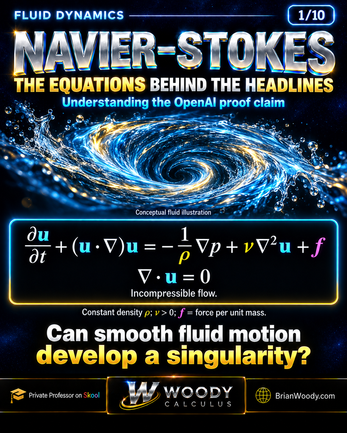

What does Navier–Stokes actually say—and what does the OpenAI announcement claim? Decode every term, verify exact fluid solutions, calculate energy decay, and test your understanding with 12 worked practice problems.
What does Navier–Stokes actually say—and what does the OpenAI announcement claim? Decode every term, verify exact fluid solutions, calculate energy decay, and test your understanding with 12 worked practice problems.
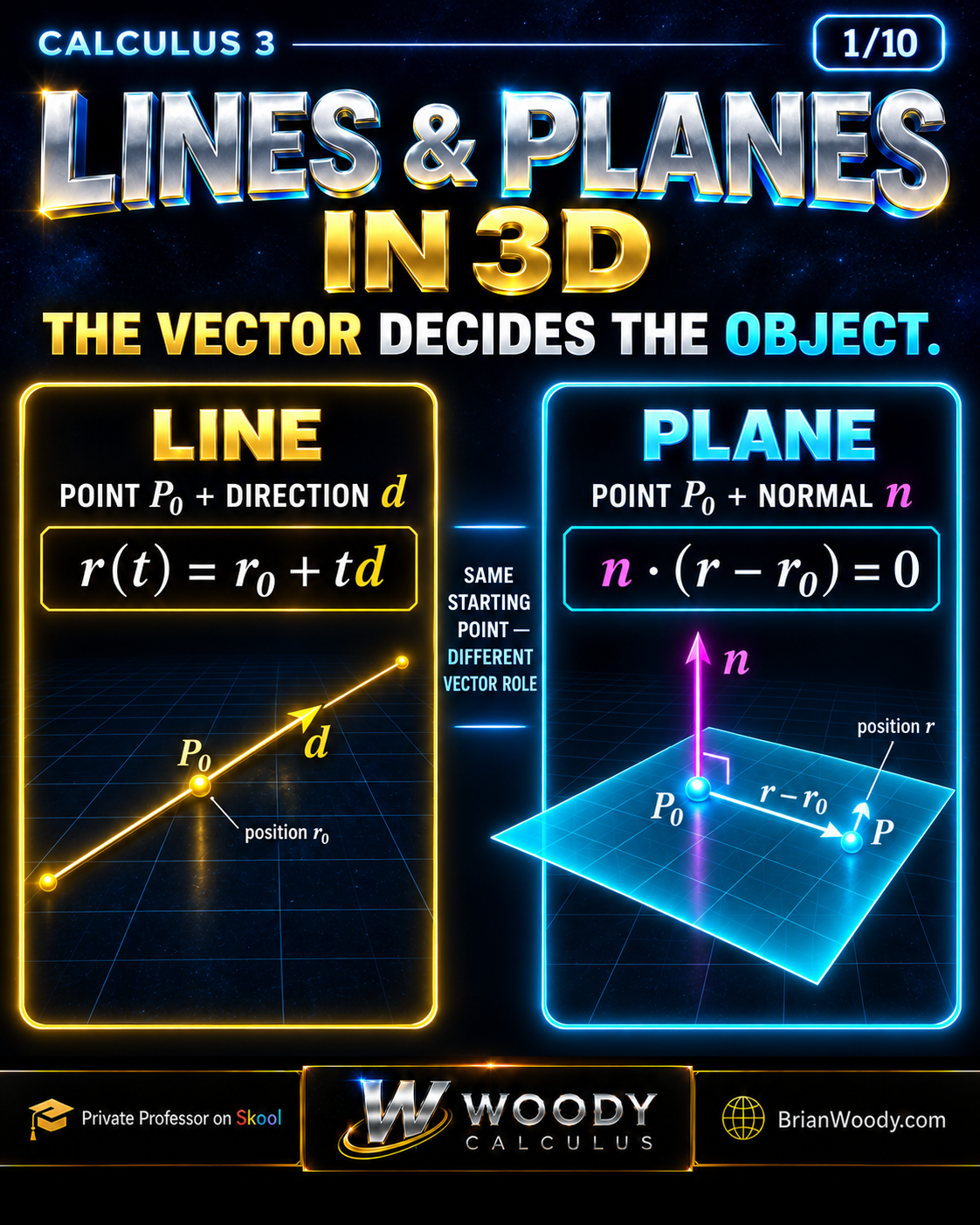
Learn how points, direction vectors, and normal vectors build lines and planes in three dimensions. Work through equations, intersections, distances, and tangent-plane normals with 10 visual slides and 12 practice problems with solutions.
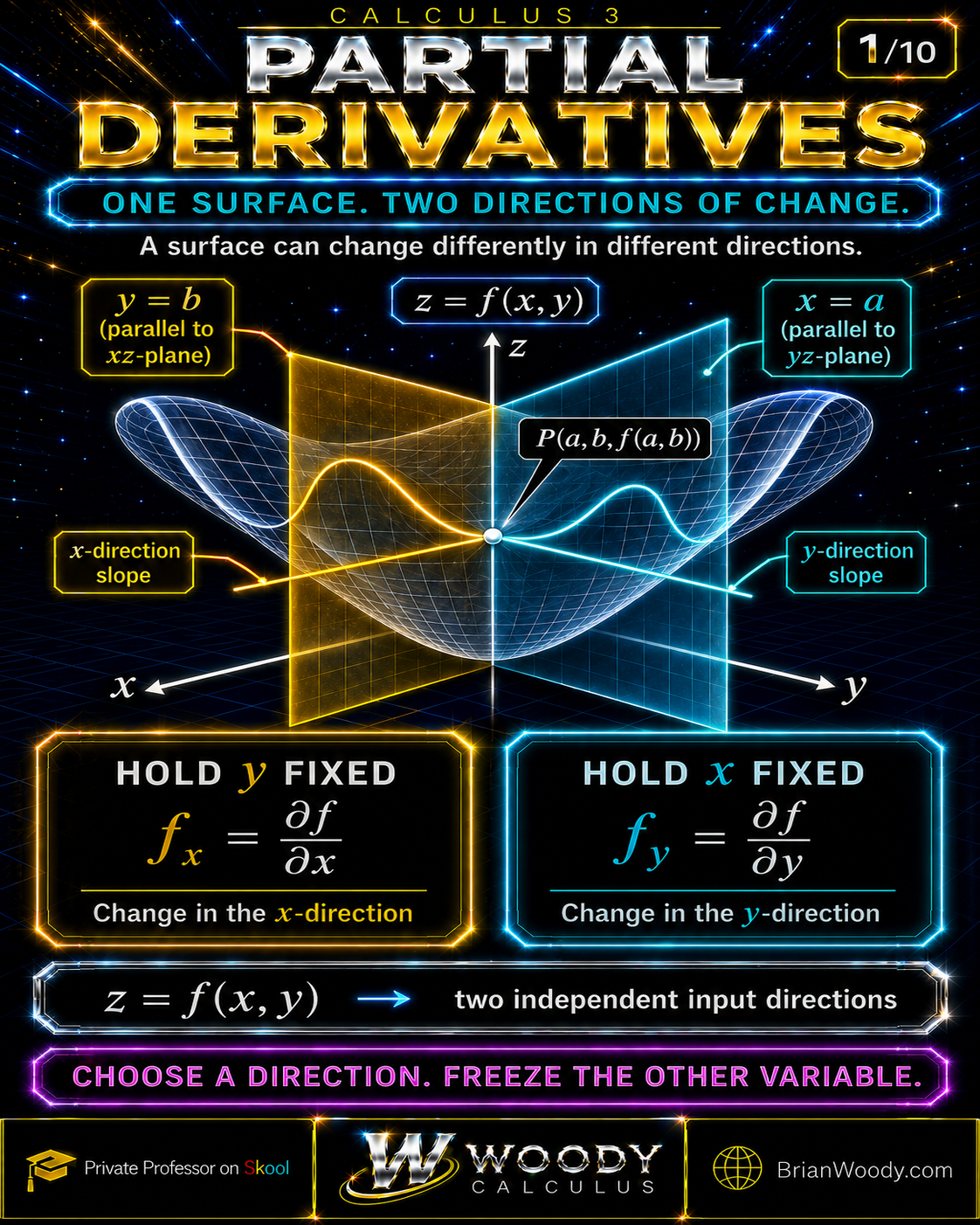
Partial derivatives measure how a multivariable function changes when one input varies and the others are held constant. This complete Calculus 3 lesson develops limit definitions, trace curves, first and mixed partials, tangent planes, the multivariable chain rule, linear approximation, rigorous counterexamples, and solved practice problems.
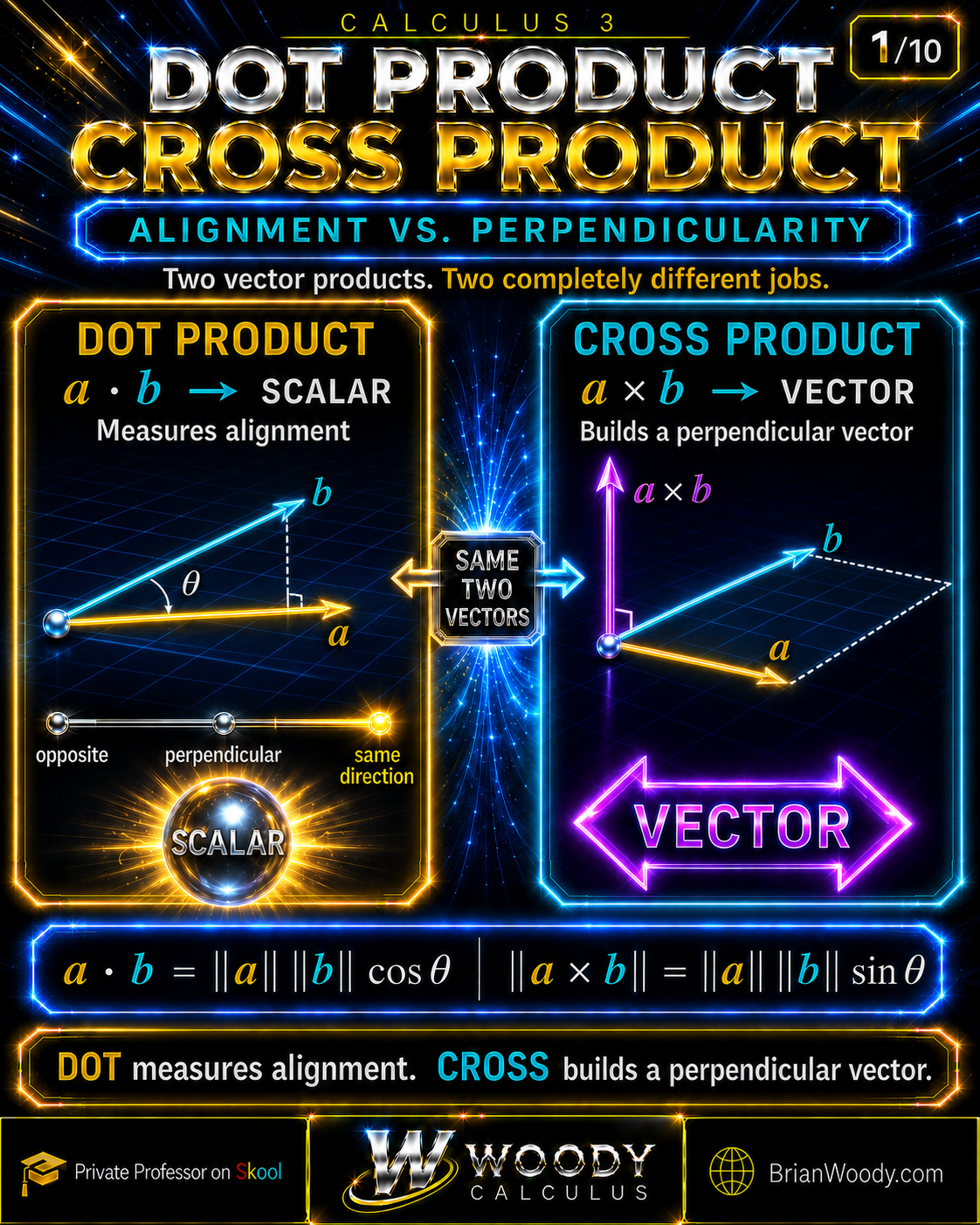
The dot product returns a scalar that measures alignment, while the cross product returns a vector perpendicular to two three-dimensional vectors. Learn the formulas, geometric meaning, right-hand rule, projections, work, area, plane normals, torque, flux, scalar triple products, Lagrange’s identity, and complete worked examples.

Triple integrals become manageable when you see the solid first. Learn how to choose a projection, write valid Cartesian bounds, integrate inside out, change the order of integration, and calculate volume, mass, average value, and center of mass through exact worked examples.
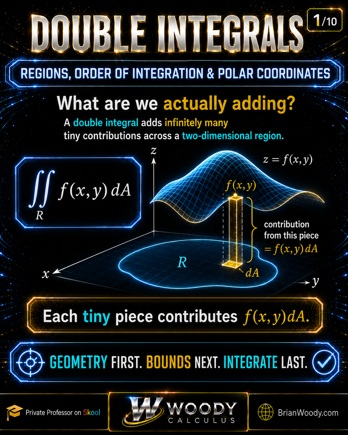
This complete Woody Calculus lesson explains double integrals from the ground up. Learn the geometric meaning of ∬R f(x,y) dA, how Fubini’s Theorem turns double integrals into iterated integrals, how to identify Type I and Type II regions, how to reverse the order of integration, and when polar coordinates make the setup easier.
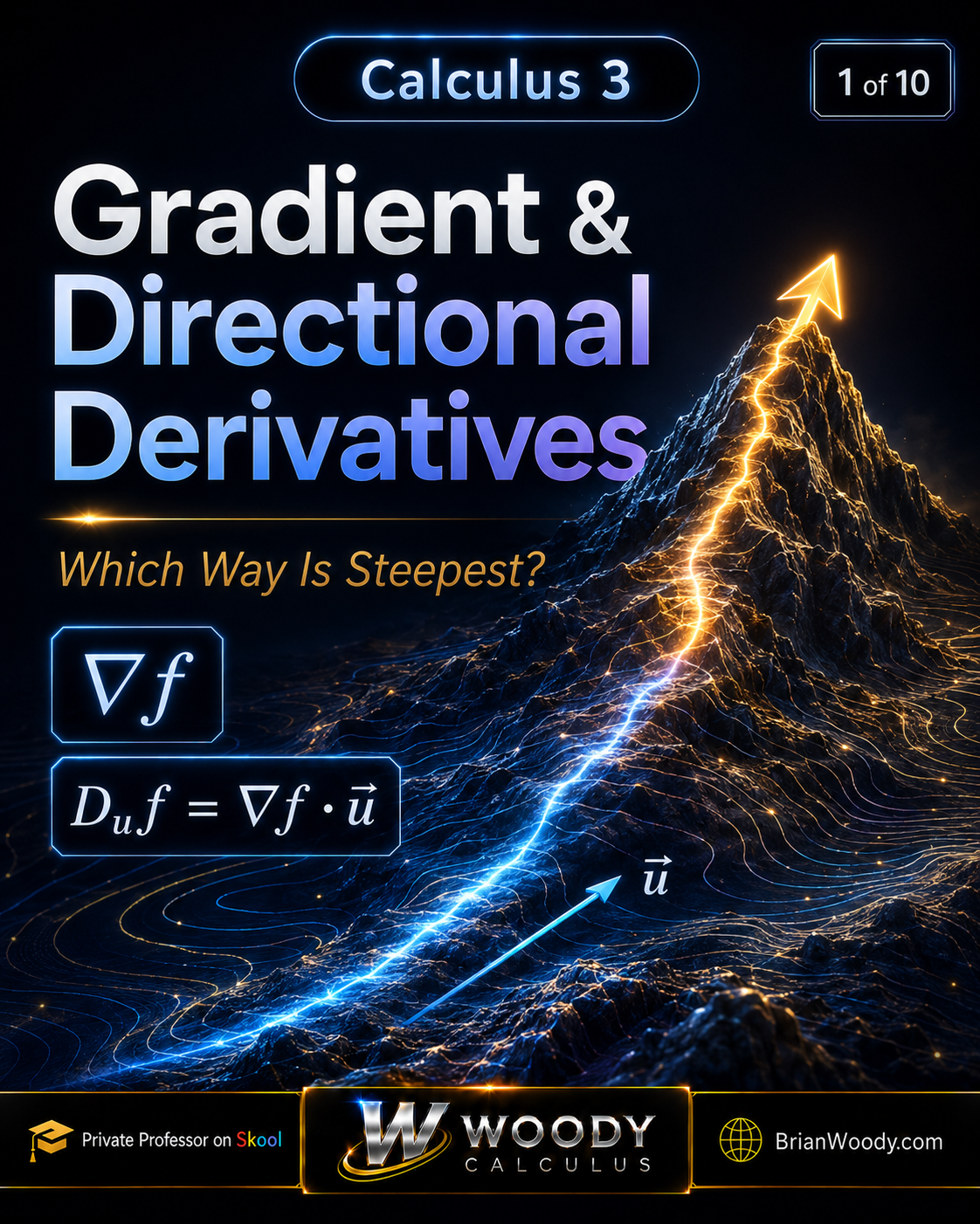
Which direction makes a multivariable function increase fastest? Learn how the gradient packages partial derivatives, how to calculate directional derivatives with unit vectors and dot products, and why gradients cross level curves at right angles.

Master cylindrical and spherical coordinates through visual geometry, conversion formulas, Jacobians, bounds, and worked triple integrals. This Calculus 3 lesson compares both systems, solves an upper hemisphere in two ways, and shows how symmetry determines the best coordinates.

The Divergence Theorem converts outward flux through a closed surface into a triple integral of divergence over the enclosed solid. Learn the theorem’s conditions, flux and divergence meanings, method-selection rules, singularity warnings, and a complete sphere example with exact verification.

Why do gradients become parallel in constrained optimization? This Woody Calculus lesson explains the geometry and algebra of Lagrange multipliers, derives the system ∇f = λ∇g, and solves complete rectangle and box optimization examples.