Calculus 3 • Multivariable Calculus
Visual lesson • Worked examples • Exam strategy • 25–30 minute study guide
Which Direction Makes a Function Increase Fastest?
In single-variable calculus, there are only two directions to move: left or right.
In multivariable calculus, there are infinitely many directions. That creates a new
question: which direction makes the function increase fastest?
The answer is the gradient. Once you know the gradient, a
directional derivative tells you how quickly the function changes
in any particular unit direction.
The Big Idea
\nabla f(a,b)
=
\left\langle
f_x(a,b),
f_y(a,b)
\right\rangle
\]
The gradient is a vector pointing toward the fastest local increase.
D_{\vec u}f(a,b)
=
\nabla f(a,b)\cdot\vec u,
\qquad
\|\vec u\|=1.
\]
The directional derivative is a scalar telling you the rate of change in
the direction you selected.
Prerequisites: What You Should Know First
You do not need to be perfect at every prerequisite. You only need enough
familiarity to recognize the pieces when they appear.
Be able to compute \(f_x\) and \(f_y\) while treating the other variable as constant.
Know how to compute \(\|\vec v\|\) and turn a nonzero vector into a unit vector.
Remember that a dot product measures directional alignment and produces a scalar.
The chain rule explains why the directional derivative becomes a gradient dot product.
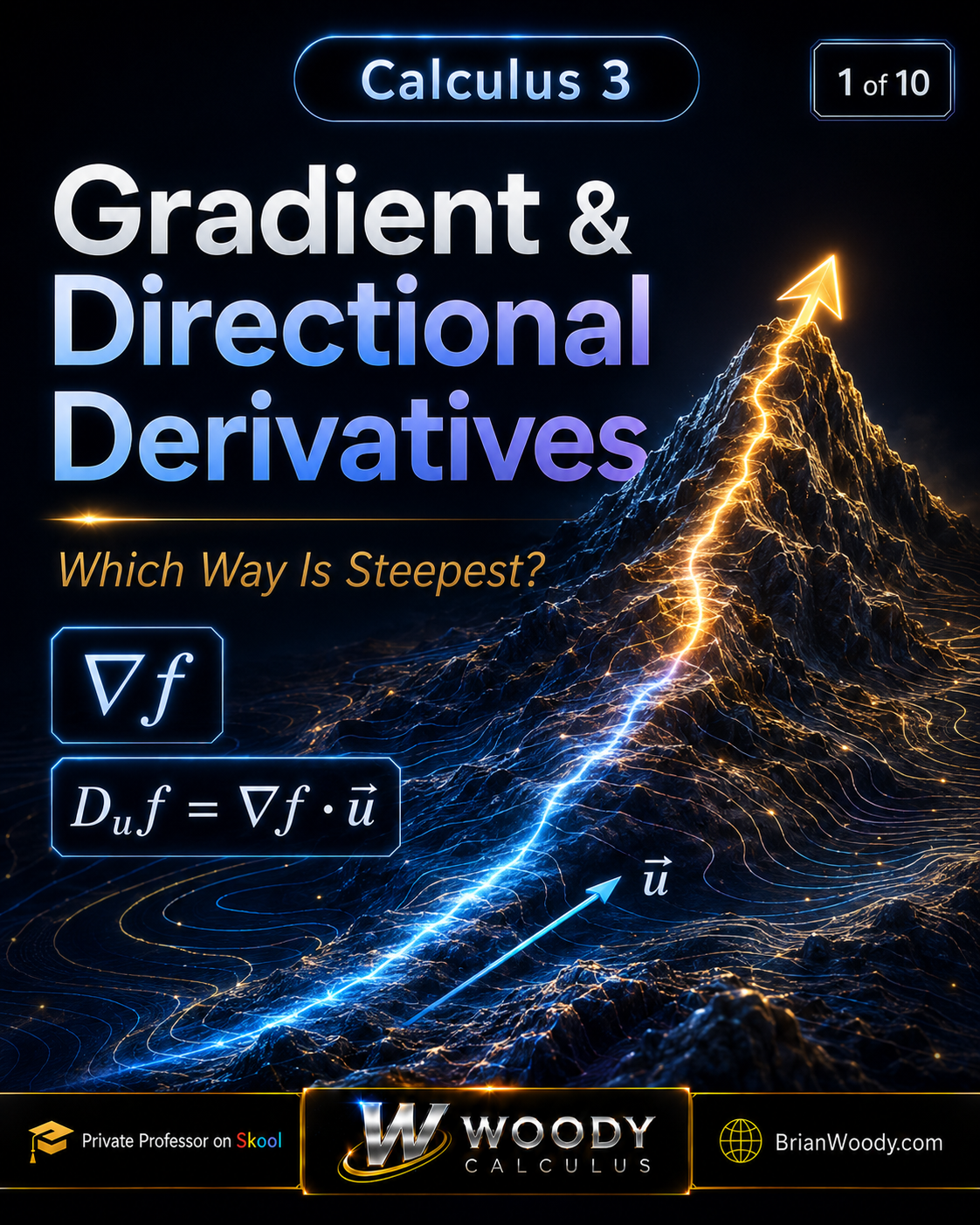
the gradient chooses the steepest climb while the directional derivative
measures the rate in a direction you choose.
What Is the Gradient?
Start with a differentiable function \(f(x,y)\). Its first partial derivatives
measure change in the coordinate directions:
f_x(x,y)=\frac{\partial f}{\partial x},
\qquad
f_y(x,y)=\frac{\partial f}{\partial y}.
\]
The gradient places those two rates into a single vector:
\boxed{
\nabla f(x,y)
=
\left\langle
f_x(x,y),
f_y(x,y)
\right\rangle
}.
\]
The two partial derivatives tell you what happens along the coordinate axes.
The gradient combines that information and answers a more powerful question:
which direction gives the greatest local increase?
Where Does the Gradient Actually Live?
If \(z=f(x,y)\), the graph of the function is a surface in three-dimensional
space. But the vector
\(\nabla f(a,b)\) lives in the two-dimensional input plane.
Think of a mountain and its hiking map. The mountain has height, but your
compass direction lies flat on the map. The gradient is that compass arrow:
it tells you which way to move across the \(xy\)-plane to climb fastest.
Another useful picture is to shine a flashlight straight down on the mountain.
The contour map is the shadow on the floor. The gradient lives on that floor,
not sticking out of the mountain surface.
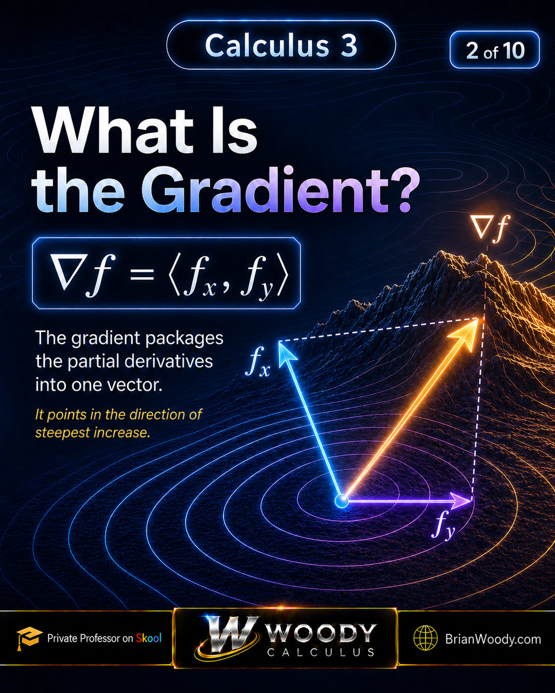
Its direction gives the fastest local increase.
What Is a Directional Derivative?
The partial derivatives \(f_x\) and \(f_y\) tell you how \(f\) changes along
the coordinate axes. But suppose you want to move northeast, southwest, or in
some completely arbitrary direction.
That is what the directional derivative measures.
\boxed{
D_{\vec u}f(a,b)
=
\nabla f(a,b)\cdot\vec u
},
\qquad
\|\vec u\|=1.
\]
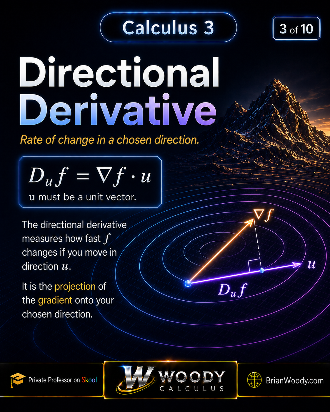
The result is a scalar. It tells you how rapidly the function
changes per unit distance as you move from the point in direction \(\vec u\).
Useful notation:
Your textbook may write the directional derivative as
\(D_{\vec u}f,\quad \nabla_{\vec u}f,\quad \text{or}\quad \partial f/\partial \vec u\).
These notations represent the same directional rate of change.
Why Does the Dot Product Appear?
Suppose you start at \((a,b)\) and move along the line determined by the
unit vector
\(\vec u=\langle u_1,u_2\rangle\).
\vec r(t)
=
\langle a,b\rangle+t\vec u
=
\langle a+tu_1,\;b+tu_2\rangle.
\]
Now restrict the multivariable function to that line:
g(t)
=
f(a+tu_1,\;b+tu_2).
\]
The multivariable chain rule gives
g^{\prime}(0)
=
f_x(a,b)u_1
+
f_y(a,b)u_2
=
\nabla f(a,b)\cdot\vec u.
\]
So the directional derivative is really an ordinary derivative taken along a
carefully chosen path through the domain.
Why Must the Direction Be a Unit Vector?
A directional derivative should measure change based on
direction alone. The length of the vector should not artificially
make the answer larger or smaller.
If a problem gives a nonzero direction vector \(\vec v\), normalize it:
\boxed{
\vec u
=
\frac{\vec v}{\|\vec v\|}
}.
\]
For
\(\vec v=\langle v_1,v_2\rangle\),
\|\vec v\|
=
\sqrt{v_1^2+v_2^2}.
\]
if the problem gives a direction vector or gives two points that determine a
direction, do not immediately take the dot product. Check the length first.
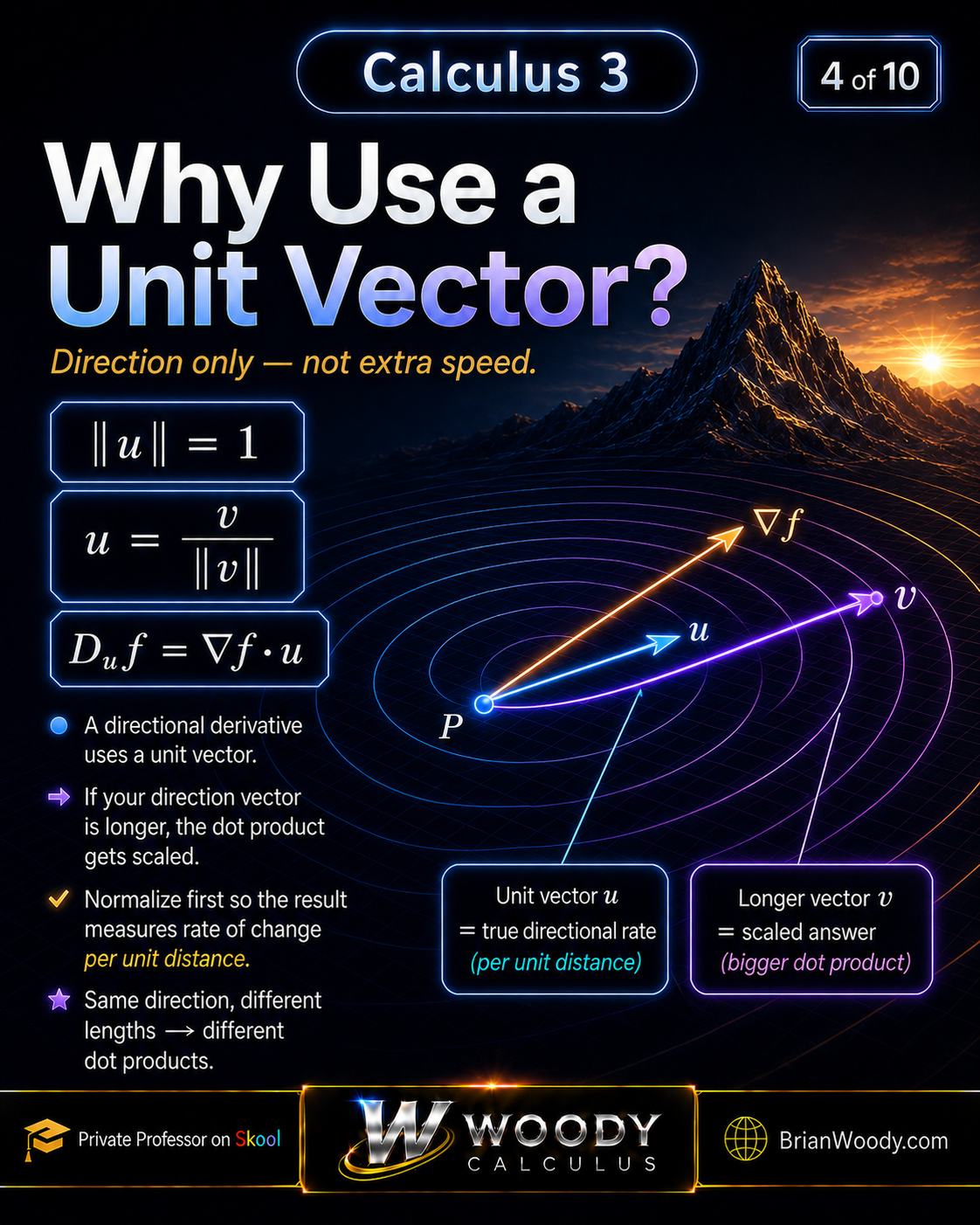
That makes the directional derivative a rate of change per unit distance.
Complete Worked Example
Let
f(x,y)=x^2+xy+y^2.
\]
Find the directional derivative at \((1,2)\) in the direction
\vec u
=
\left\langle
\frac35,
\frac45
\right\rangle.
\]
Build the Gradient
f_x=2x+y,
\qquad
f_y=x+2y.
\]
\nabla f(x,y)
=
\langle2x+y,\;x+2y\rangle.
\]
Evaluate at the Point
\begin{aligned}
\nabla f(1,2)
&=
\langle2(1)+2,\;1+2(2)\rangle\\
&=
\boxed{\langle4,5\rangle}.
\end{aligned}
\]
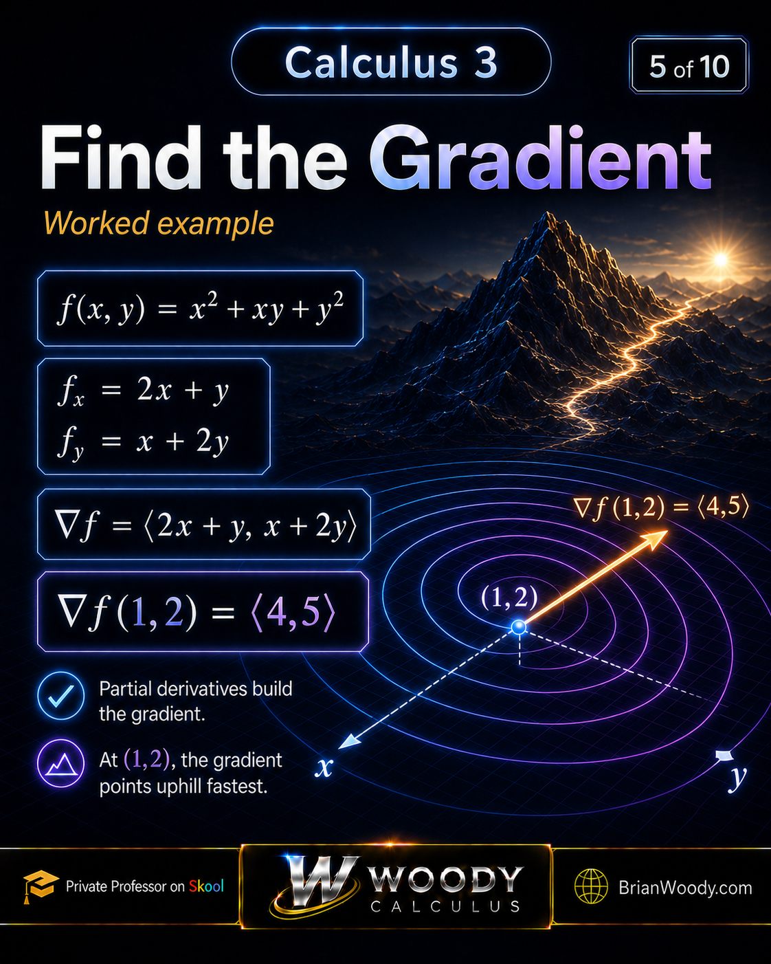
\(\langle4,5\rangle\).
Check the Direction
\left\|
\left\langle
\frac35,\frac45
\right\rangle
\right\|
=
\sqrt{
\frac9{25}
+
\frac{16}{25}
}
=
1.
\]
Good. The supplied vector is already a unit vector.
Take the Dot Product
\begin{aligned}
D_{\vec u}f(1,2)
&=
\langle4,5\rangle
\cdot
\left\langle
\frac35,\frac45
\right\rangle\\
&=
4\left(\frac35\right)
+
5\left(\frac45\right)\\
&=
\frac{12}{5}
+
\frac{20}{5}\\
&=
\boxed{\frac{32}{5}}.
\end{aligned}
\]
Because \(32/5>0\), the function increases as you move from \((1,2)\)
in the chosen direction.
Verify the Answer
\|\nabla f(1,2)\|
=
\sqrt{4^2+5^2}
=
\sqrt{41}
\approx6.403.
\]
Since
\[
\frac{32}{5}=6.4,
\]
the selected direction is almost perfectly aligned with the gradient.
That is why the directional rate is almost equal to the maximum possible rate.
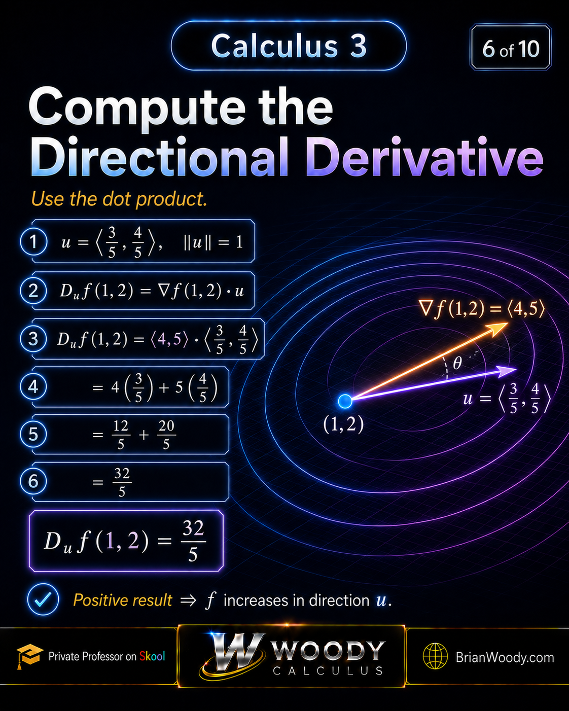
\(\boxed{32/5}\), so the function is increasing in the chosen direction.
professors often reuse the same gradient in several parts of a problem.
You may find the gradient, then use it for a directional derivative,
a tangent plane, a normal direction, or an optimization question.
Try It Yourself
This problem deliberately gives you a direction that is
not a unit vector.
\(f(x,y)=x^2y\),
find the directional derivative at \((2,1)\) in the direction
\(\langle1,1\rangle\).
Show the complete solution
First compute the gradient:
\nabla f(x,y)
=
\langle2xy,\;x^2\rangle.
\]
At \((2,1)\),
\nabla f(2,1)
=
\langle4,4\rangle.
\]
Normalize the direction:
\vec u
=
\left\langle
\frac1{\sqrt2},
\frac1{\sqrt2}
\right\rangle.
\]
Now take the dot product:
\begin{aligned}
D_{\vec u}f(2,1)
&=
\langle4,4\rangle
\cdot
\left\langle
\frac1{\sqrt2},
\frac1{\sqrt2}
\right\rangle\\
&=
\boxed{4\sqrt2}.
\end{aligned}
\]
Notice something even better:
\(\langle1,1\rangle\) points in exactly the same direction as
\(\langle4,4\rangle\). Therefore the chosen direction is the gradient
direction itself, so the answer should equal
\(\|\nabla f(2,1)\|=4\sqrt2\).
What Does the Sign of a Directional Derivative Mean?
\(D_{\vec u}f>0\) means the function increases in direction \(\vec u\).
\(D_{\vec u}f<0\) means the function decreases in direction \(\vec u\).
\(D_{\vec u}f=0\) means there is no first-order change in that direction.
A zero directional derivative does not mean the entire function
is constant. It only describes what happens locally at the chosen point in the
chosen direction.
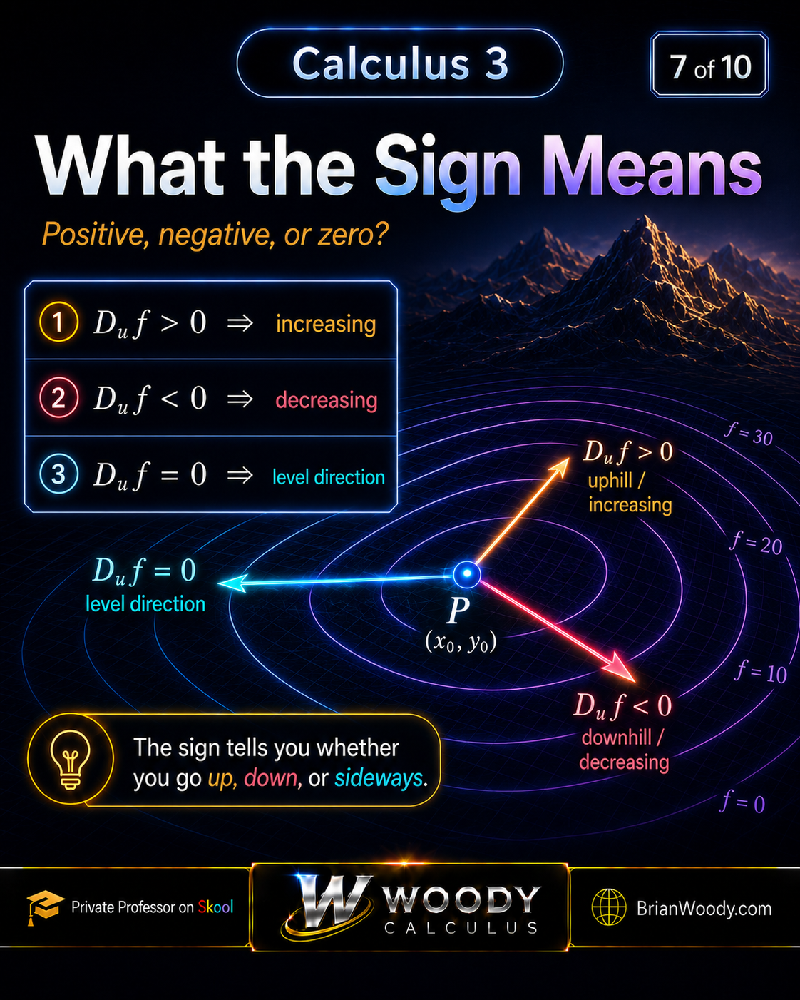
uphill, downhill, or locally sideways.
Fastest Increase and Steepest Decrease
The dot-product formula can also be written using the angle \(\theta\)
between the gradient and the unit direction:
\boxed{
D_{\vec u}f
=
\|\nabla f\|\cos\theta
}.
\]
This one equation explains the geometry of the entire topic.
| Angle | Directional derivative | Meaning |
|---|---|---|
| \(0^\circ\) | \(\|\nabla f\|\) | Fastest possible increase |
| \(60^\circ\) | \(\frac12\|\nabla f\|\) | Increasing, but more slowly |
| \(90^\circ\) | \(0\) | No first-order change |
| \(120^\circ\) | \(-\frac12\|\nabla f\|\) | Decreasing |
| \(180^\circ\) | \(-\|\nabla f\|\) | Steepest possible decrease |
Direction of Fastest Increase
\boxed{
\vec u_{\max}
=
\frac{\nabla f}{\|\nabla f\|}
}
\]
\boxed{
\max_{\|\vec u\|=1}
D_{\vec u}f
=
\|\nabla f\|
}.
\]
Direction of Steepest Decrease
\boxed{
\vec u_{\min}
=
-\frac{\nabla f}{\|\nabla f\|}
}
\]
\boxed{
\min_{\|\vec u\|=1}
D_{\vec u}f
=
-\|\nabla f\|
}.
\]
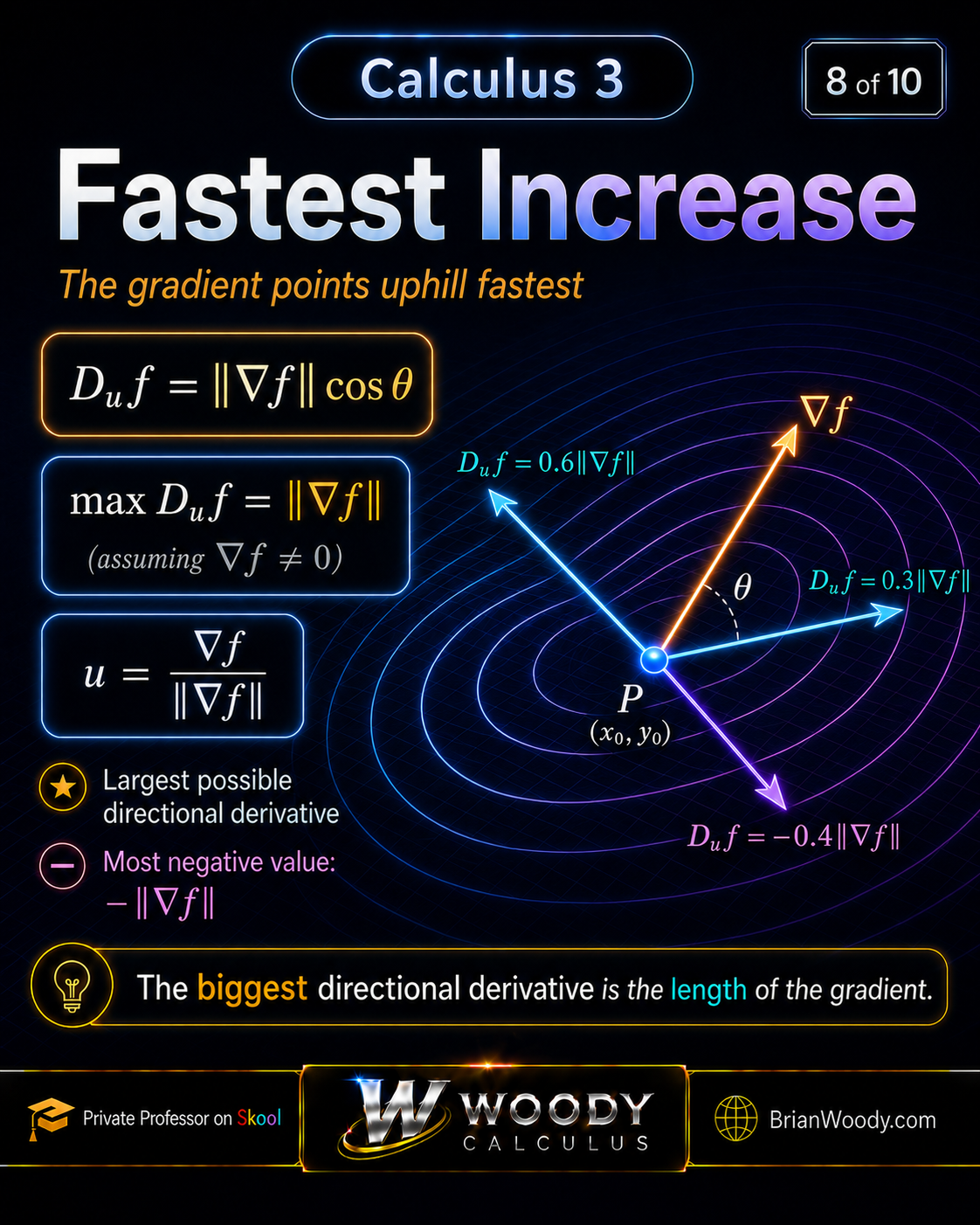
Why Machine Learning Uses the Negative Gradient
This Calculus 3 idea extends far beyond a calculus exam.
It is also one of the central ideas behind optimization and machine learning.
Suppose a model has a loss function
\(L(\boldsymbol\theta)\).
The gradient
\(\nabla L(\boldsymbol\theta)\)
points toward the direction in parameter space where the loss increases fastest.
If the goal is to make the loss smaller, we move in the opposite direction.
\boxed{
\boldsymbol\theta_{k+1}
=
\boldsymbol\theta_k
–
\eta
\nabla L(\boldsymbol\theta_k)
}.
\]
Read the Formula in Plain English
Start with the model’s current parameters.
Compute the gradient of the loss there.
Reverse that direction using the minus sign.
Then scale the step by the learning rate \(\eta\).
The gradient tells the model which way the error rises fastest.
The negative gradient sends the model toward lower error.
There is one useful distinction:
the unit direction of steepest decrease is
-\frac{\nabla L}{\|\nabla L\|}.
\]
Standard gradient descent normally uses the full vector
\(-\nabla L\) instead. The learning rate controls how large the actual
parameter update is.
So the same geometry students learn here appears again in numerical optimization,
statistics, artificial intelligence, and neural-network training.
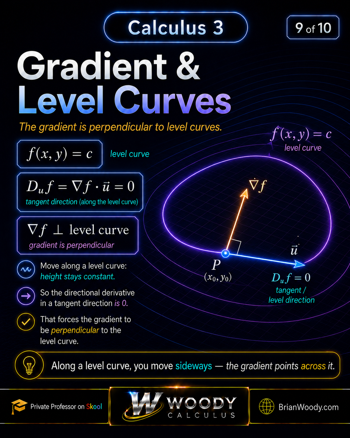
Why Is the Gradient Perpendicular to Level Curves?
A level curve is defined by
f(x,y)=c,
\]
where \(c\) is constant.
Suppose
\(\vec r(t)\)
traces a path along that level curve. Because the function remains constant,
f(\vec r(t))=c.
\]
Differentiate using the chain rule:
\frac{d}{dt}
f(\vec r(t))
=
\nabla f(\vec r(t))
\cdot
\vec r^{\,\prime}(t)
=
0.
\]
The vector
\(\vec r^{\,\prime}(t)\)
points tangent to the level curve. Its dot product with the gradient is zero,
so the gradient is perpendicular to the tangent direction.
\boxed{
\nabla f
\perp
\text{a regular level curve}
}.
\]
Your height stays constant. To change height fastest, you need to cut across
the contour lines. That is exactly what the gradient does.
This geometry is also the foundation of
Lagrange multipliers
.
What Changes in Three Dimensions?
Almost nothing changes conceptually.
For a differentiable function \(f(x,y,z)\),
\boxed{
\nabla f(x,y,z)
=
\langle
f_x,
f_y,
f_z
\rangle
}.
\]
For a unit vector
\(\vec u=\langle u_1,u_2,u_3\rangle\),
D_{\vec u}f
=
\nabla f\cdot\vec u
=
f_xu_1+f_yu_2+f_zu_3.
\]
The gradient still points toward fastest increase.
The negative gradient still points toward fastest decrease.
And the gradient is normal to a regular level surface
\(f(x,y,z)=c\).
Professor Woody’s Exam Method
Do not begin by searching your memory for a formula.
First decide what mathematical object the problem is asking for.
Choose the Method Before You Calculate
Compute the first partial derivatives and assemble them into
\(\nabla f\).
Build or identify the direction vector, normalize it, then compute
\(\nabla f\cdot\vec u\).
Compute
\(\|\nabla f\|\).
Normalize the gradient:
\(\nabla f/\|\nabla f\|\).
Move opposite the gradient:
\(-\nabla f/\|\nabla f\|\).
Use the nonzero gradient vector itself.
A Reliable Workflow for Directional-Derivative Problems
Compute the gradient → evaluate at the point → build the direction →
normalize it → take the dot product → interpret the sign → check the magnitude.
A correct directional derivative using a unit vector must satisfy
\boxed{
|D_{\vec u}f|
\leq
\|\nabla f\|
}.
\]
If your absolute value is larger than the gradient magnitude,
something went wrong.
Quick-Reference Exam Table
| Question asks for… | Use… | Watch out for… |
|---|---|---|
| Gradient at a point | \(\nabla f=\langle f_x,f_y\rangle\) | The answer is a vector |
| Rate in a chosen direction | \(\nabla f\cdot\vec u\) | Make sure \(\|\vec u\|=1\) |
| Maximum rate | \(\|\nabla f\|\) | The answer is a scalar |
| Direction of fastest increase | \(\nabla f/\|\nabla f\|\) | The answer is a unit vector |
| Direction of steepest decrease | \(-\nabla f/\|\nabla f\|\) | Do not lose the minus sign |
| Normal to a regular level curve | \(\nabla f\) | Require \(\nabla f\neq\vec0\) |
How This Connects to the Rest of Calculus 3
Gradients and directional derivatives are not isolated formulas.
They become structural tools throughout multivariable and vector calculus.
Lagrange Multipliers
At a constrained optimum, gradients become parallel because the gradient
points normal to the relevant level curves and constraint.
The same partial derivatives forming the gradient determine the best local
linear approximation to a surface.
Line Integrals and Vector Fields
Dot products again measure how much of a vector field points along a
direction of motion.
When
\(\mathbf F=\nabla f\),
the scalar function \(f\) acts as a potential function.
Jacobians and Change of Variables
The gradient measures local change in a scalar function, while the Jacobian
generalizes derivative information to multivariable mappings.
Cylindrical and Spherical Coordinates
Later vector-calculus formulas depend on understanding how directions and
scale change in different coordinate systems.
Common Mistakes That Cost Points
If \(\vec v\) is not a unit vector, first compute
\(\vec u=\vec v/\|\vec v\|\).
The gradient is a vector. The directional derivative is a scalar.
Find the symbolic partial derivatives first, build the gradient, then
evaluate at the point.
\(\nabla f/\|\nabla f\|\) is the fastest unit direction.
\(\|\nabla f\|\) is the maximum rate.
After calculating the directional derivative, say whether the function
increases, decreases, or has zero first-order change.
For a unit direction,
\(|D_{\vec u}f|\leq\|\nabla f\|\).
Use this as a fast exam check.
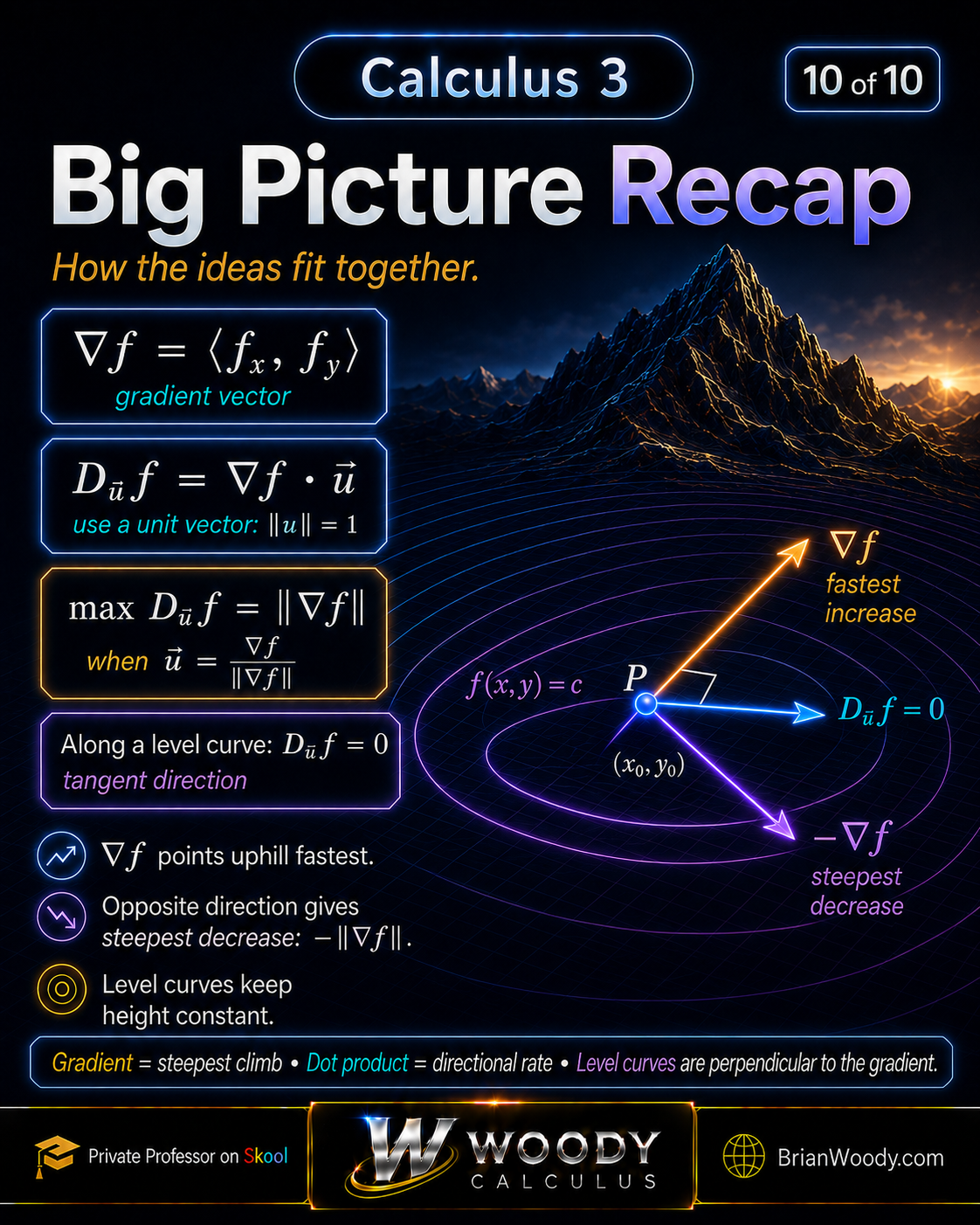
the gradient gives the steepest climb, the dot product gives the selected
directional rate, and level curves are perpendicular to the gradient at regular points.
Gradient and Directional Derivative FAQ
What is the gradient of a function?
For a differentiable function \(f(x,y)\),
\[
\nabla f=\langle f_x,f_y\rangle.
\]
It points toward the fastest local increase.
How do you calculate a directional derivative?
Find the gradient, evaluate it at the point, normalize the chosen direction,
and compute
\[
D_{\vec u}f=\nabla f\cdot\vec u.
\]
Why does the direction vector need to be a unit vector?
Normalizing removes the effect of vector length so the result measures
change per unit distance.
What does a positive directional derivative mean?
The function increases locally in that direction.
What does a negative directional derivative mean?
The function decreases locally in that direction.
What does a zero directional derivative mean?
There is no first-order change in that direction at the selected point.
What direction gives the maximum directional derivative?
If \(\nabla f\neq\vec0\), the maximizing unit direction is
\[
\frac{\nabla f}{\|\nabla f\|},
\]
and the maximum value is
\(\|\nabla f\|\).
What direction gives the steepest decrease?
The direction is
\[
-\frac{\nabla f}{\|\nabla f\|},
\]
and the minimum directional derivative is
\(-\|\nabla f\|\).
Why is the gradient perpendicular to a level curve?
Moving tangent to a level curve keeps the function constant. Therefore the
tangent directional derivative is zero, which means the tangent direction
has zero dot product with the gradient.
What happens when the gradient is zero?
Every directional derivative is zero at that point. More analysis is needed
to determine whether the point is a maximum, minimum, saddle point, or
another type of critical point.
How is the gradient used in machine learning?
The gradient points toward increasing loss. Gradient descent moves in the
negative-gradient direction so the model can reduce that loss.
Additional University Resources
MIT OpenCourseWare: Gradient and Level Curves
Review the gradient definition and its relationship with level curves.
MIT OpenCourseWare: Directional Derivatives
Review directional derivative examples and additional university-level practice.
UC Berkeley Math 53
Explore additional multivariable calculus lecture material.
Google Machine Learning Crash Course: Gradient Descent
See how the negative-gradient idea becomes an optimization algorithm.
Do Not Stay Stuck
Bring Your Actual Calculus 3 Problems Into the Mastery Lab
If a directional derivative, tangent plane, level-curve, or optimization
problem is giving you trouble, bring the exact problem and your attempted
work into the Woody Calculus community. The goal is not just to finish one
problem—it is to identify the structure so you can do the next one yourself.
Professor-Led Calculus 3 Training
Turn the Formula Into a Method You Can Use Under Pressure
The goal is not to memorize one more equation.
The goal is to recognize the problem type, choose the correct mathematical object,
organize the solution, verify it, and explain what the answer means.
That same process carries forward into tangent planes, optimization,
multiple integrals, vector fields, line integrals, surface integrals,
Green’s Theorem, Stokes’ Theorem, and the Divergence Theorem.