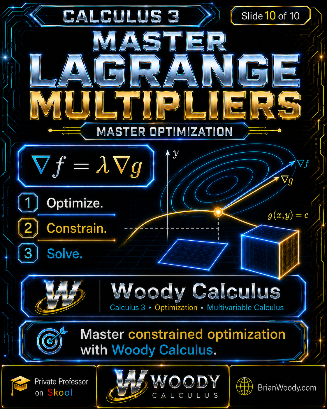
Lagrange multipliers are a Calculus 3 method for maximizing or minimizing a multivariable function while satisfying an equality constraint.
If the objective function is \(f(x,y)\) and the constraint is
\(g(x,y)=c\), the central equation is:
\boxed{
\nabla f=\lambda\nabla g.
}
\]
This equation says that, at a regular constrained maximum or minimum, the objective gradient and constraint gradient are scalar multiples of one another.
When both gradients are nonzero, they point in parallel or opposite directions. Geometrically, the best attainable level curve of \(f\) is tangent to the constraint curve.
A constrained optimum occurs where the objective cannot improve without leaving the constraint.
That is the real idea behind Lagrange multipliers. The method is not an arbitrary collection of partial derivatives. It is a geometric statement about:
- level curves,
- tangent directions,
- normal vectors,
- gradients,
- and the directions in which movement is allowed.
This Woody Calculus lesson explains why the gradients become parallel and then develops three complete applications:
- maximizing the area of a rectangle with fixed perimeter,
- maximizing the volume of a rectangular box with fixed surface area,
- finding the maximum and minimum of a linear objective on the unit circle.
Published: .
Last updated: .
Estimated read time: 22–26 minutes.

What Are Lagrange Multipliers?
Lagrange multipliers are a method for finding extrema of an objective function while restricting the variables to satisfy one or more constraints.
Suppose the objective is:
f(x,y),
\]
and the constraint is:
g(x,y)=c.
\]
The constraint limits the points available to the optimizer. Instead of moving anywhere in the \(xy\)-plane, we may move only along the curve \(g(x,y)=c\).
At a regular constrained extremum:
\boxed{
\nabla f(x,y)=\lambda\nabla g(x,y).
}
\]
Together with the constraint, this produces a system of three equations:
\boxed{
\begin{aligned}
f_x&=\lambda g_x,\\
f_y&=\lambda g_y,\\
g(x,y)&=c.
\end{aligned}
}
\]
Plain-language answer: Lagrange multipliers find points where the objective gradient aligns with the normal direction of the constraint.
Unconstrained vs. Constrained Optimization
An unconstrained extremum normally satisfies \(\nabla f=0\), but a constrained extremum may occur where \(\nabla f\ne0\).
Without a constraint, we may move in every direction. If \(\nabla f\ne0\), moving in the gradient direction increases \(f\), so an interior unconstrained optimum generally requires:
\nabla f=0.
\]
Under a constraint, most directions are forbidden. We may move only in directions tangent to the constraint.
The gradient of \(f\) can be nonzero while having no component in any permitted tangent direction. In that situation, \(f\) cannot improve without leaving the constraint.

Why Do the Gradients Become Parallel?
At a constrained extremum, the objective has zero directional derivative along every tangent direction allowed by the constraint.
Let \(\mathbf{T}\) be a tangent vector to the constraint curve. Because \(g\) remains constant as we move along the constraint:
\nabla g\cdot\mathbf{T}=0.
\]
Thus \(\nabla g\) is normal to the constraint.
At a constrained extremum, moving slightly in either tangent direction cannot increase or decrease the objective to first order:
\nabla f\cdot\mathbf{T}=0.
\]
Therefore, \(\nabla f\) is also normal to the same tangent direction.
In the plane, the normal direction to a regular curve is one-dimensional. Two vectors normal to the same tangent line must be scalar multiples:
\boxed{
\nabla f=\lambda\nabla g.
}
\]
When both gradients are nonzero, they are parallel or antiparallel. The sign of \(\lambda\) records which orientation occurs.
Level Curves, Tangency, and the Constraint
The best attainable level curve of the objective just touches the constraint at a regular constrained optimum.
A level curve of \(f\) has the form:
f(x,y)=k.
\]
Different values of \(k\) represent different objective values. As we move toward higher level curves, the value of \(f\) increases.
The constraint is:
g(x,y)=c.
\]
At the greatest level of \(f\) that still intersects the constraint, the level curve typically becomes tangent to the constraint curve.
Since gradients are normal to level curves, tangency forces the two gradients to lie in the same normal direction.

The Lagrange Multiplier Theorem
The standard theorem requires a smooth objective, a smooth constraint, and a nonzero constraint gradient at the candidate point.
Suppose \(f\) and \(g\) are continuously differentiable near a point \((x^*,y^*)\). Assume:
g(x^*,y^*)=c,
\]
\nabla g(x^*,y^*)\ne\mathbf{0}.
\]
If \(f\) has a local maximum or minimum on the constraint \(g=c\) at \((x^*,y^*)\), then there exists a scalar \(\lambda\) such that:
\boxed{
\nabla f(x^*,y^*)
=
\lambda\nabla g(x^*,y^*).
}
\]
How to Build the Lagrange Multiplier System
You may work directly with gradients or introduce the Lagrangian function.
For the constraint \(g(x,y)=c\), define:
\boxed{
\mathcal{L}(x,y,\lambda)
=
f(x,y)-\lambda\bigl(g(x,y)-c\bigr).
}
\]
Set every partial derivative equal to zero:
\boxed{
\mathcal{L}_x=0,
\qquad
\mathcal{L}_y=0,
\qquad
\mathcal{L}_{\lambda}=0.
}
\]
These equations are equivalent to:
\boxed{
\begin{aligned}
f_x&=\lambda g_x,\\
f_y&=\lambda g_y,\\
g(x,y)&=c.
\end{aligned}
}
\]
The gradient form is usually more geometric. The Lagrangian form is often convenient when organizing a larger system.
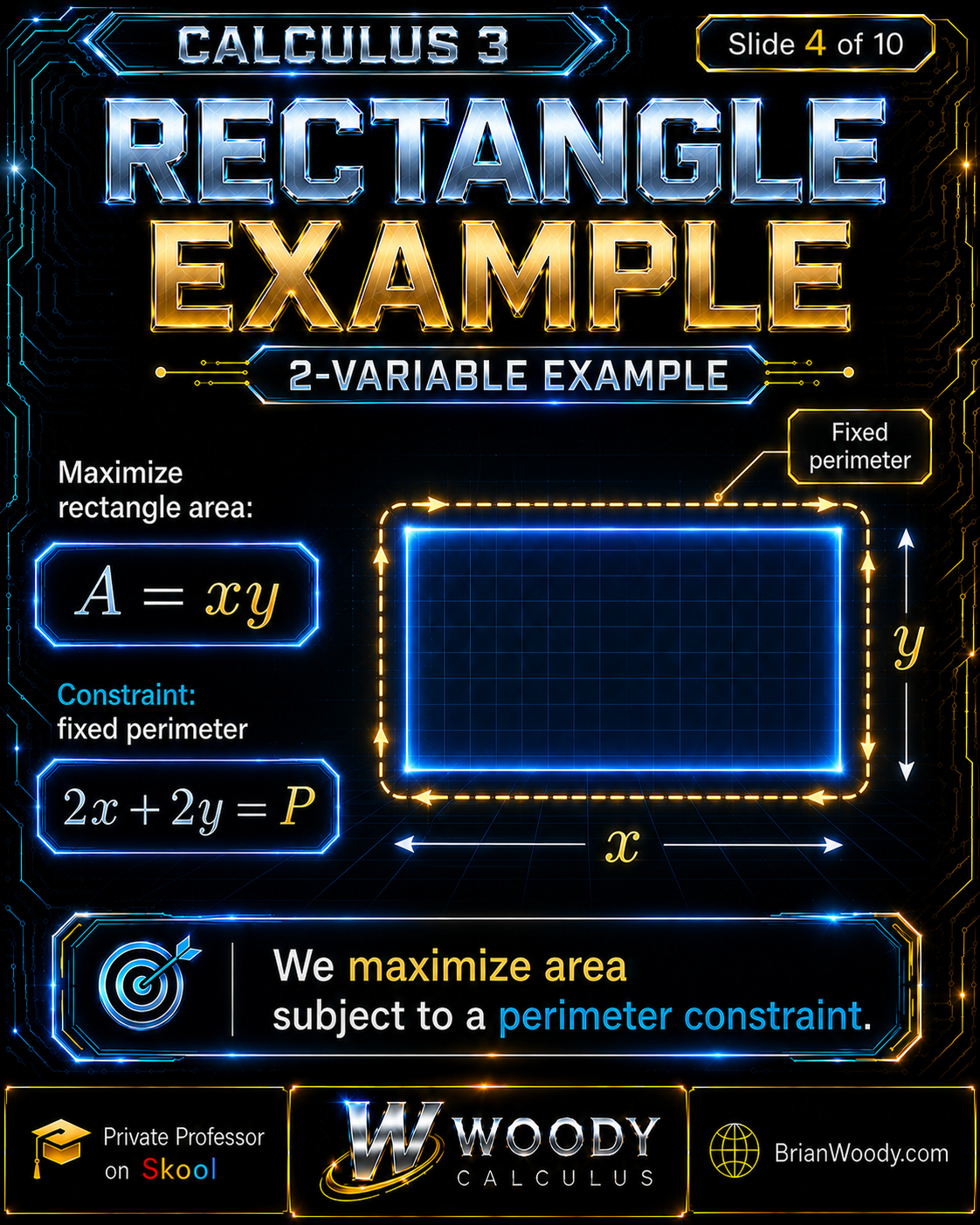
Rectangle Example: Maximize Area with Fixed Perimeter
Among all rectangles with a fixed perimeter, the square has the greatest area.
Let the rectangle have side lengths \(x>0\) and \(y>0\).
The objective function is its area:
\boxed{
A(x,y)=xy.
}
\]
Suppose the perimeter is fixed at \(P\):
\boxed{
2x+2y=P.
}
\]
Define:
g(x,y)=2x+2y.
\]
We maximize \(A\) subject to \(g=P\).
Why the Maximum-Area Rectangle Is a Square
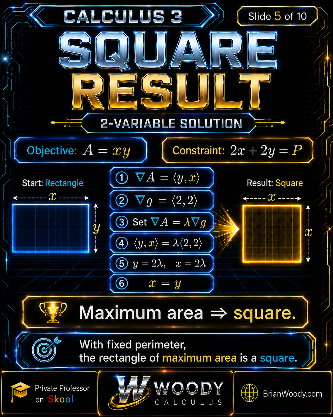
The Lagrange equations force the two side lengths to be equal.
Step 1: Compute the Gradients
\nabla A
=
\left\langle y,x\right\rangle.
\]
\nabla g
=
\left\langle2,2\right\rangle.
\]
Step 2: Set the Gradients Equal up to a Scalar
\left\langle y,x\right\rangle
=
\lambda\left\langle2,2\right\rangle.
\]
Match corresponding components:
y=2\lambda,
\qquad
x=2\lambda.
\]
Therefore:
\boxed{x=y.}
\]
Step 3: Use the Constraint
Substitute \(y=x\) into:
2x+2y=P.
\]
4x=P.
\]
Thus:
\boxed{
x=y=\frac{P}{4}.
}
\]
Step 4: Find the Maximum Area
A_{\max}
=
\left(\frac{P}{4}\right)
\left(\frac{P}{4}\right)
=
\boxed{\frac{P^2}{16}}.
\]
The maximizing rectangle has equal side lengths, so it is a square.
Plain-language answer: with fixed perimeter \(P\), the maximum-area rectangle is a square with side length \(P/4\) and area \(P^2/16\).
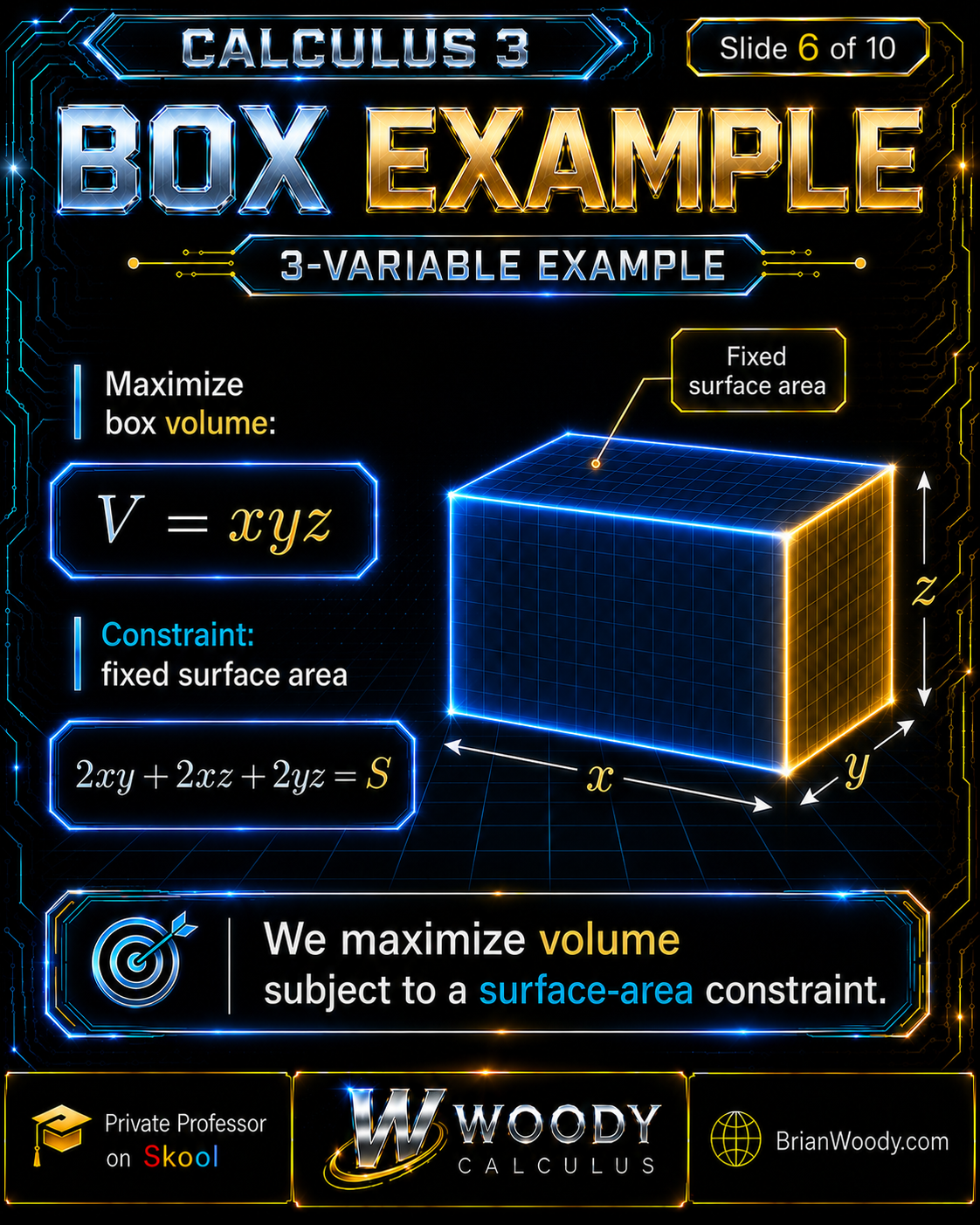
Box Example: Maximize Volume with Fixed Surface Area
Among all rectangular boxes with a fixed surface area, the cube has the greatest volume.
Let the positive side lengths be \(x\), \(y\), and \(z\).
The objective is volume:
\boxed{
V(x,y,z)=xyz.
}
\]
The surface-area constraint is:
\boxed{
2xy+2xz+2yz=S.
}
\]
Define:
g(x,y,z)=2xy+2xz+2yz.
\]
We maximize \(V\) subject to \(g=S\).
Build the Three-Variable Lagrange System
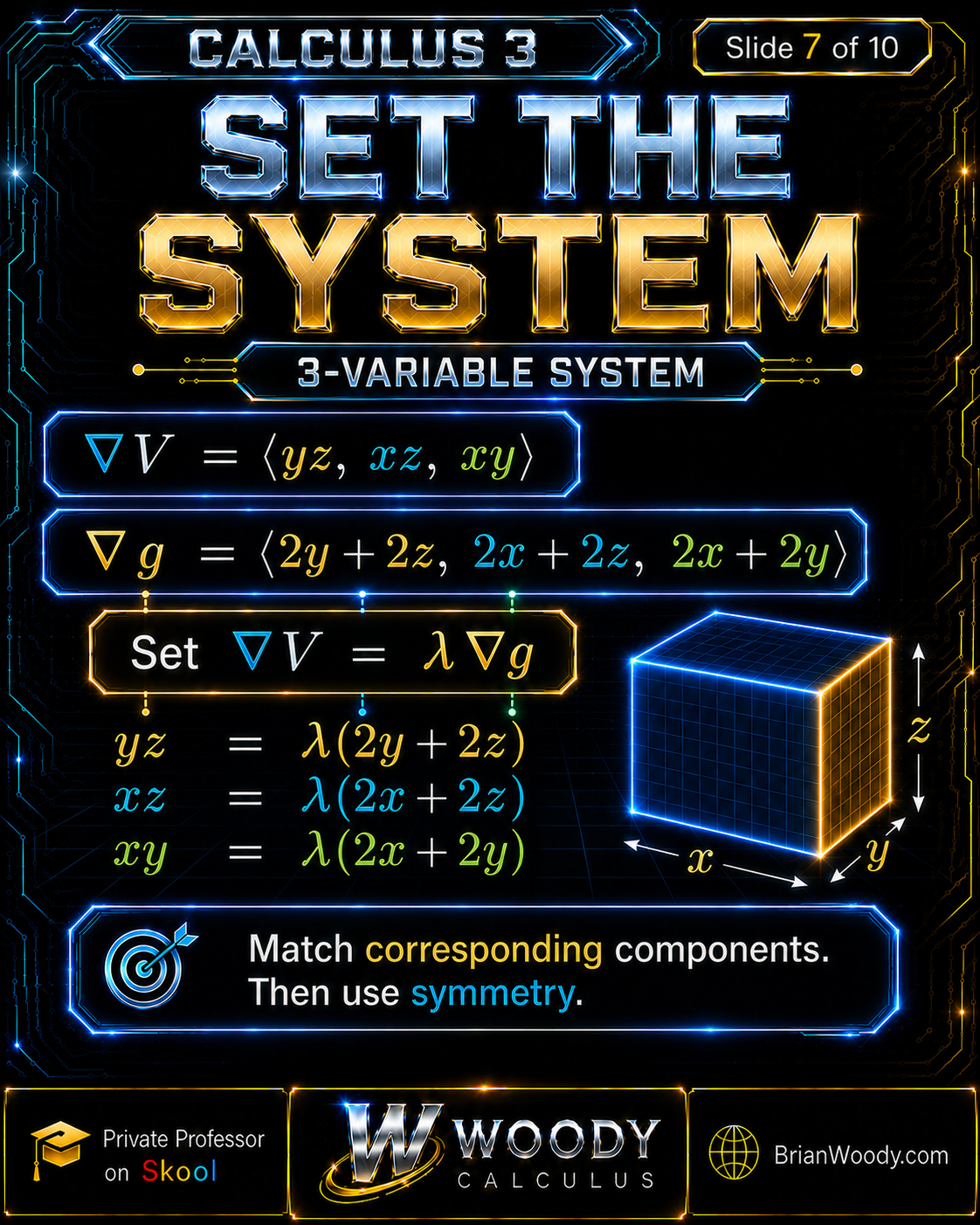
In three variables, equate the three corresponding components of the objective and constraint gradients.
Step 1: Compute the Objective Gradient
\nabla V
=
\left\langle
yz,xz,xy
\right\rangle.
\]
Step 2: Compute the Constraint Gradient
\nabla g
=
\left\langle
2y+2z,\,
2x+2z,\,
2x+2y
\right\rangle.
\]
Step 3: Set \(\nabla V=\lambda\nabla g\)
\nabla V
=
\lambda\nabla g.
\]
Matching components gives:
\boxed{
\begin{aligned}
yz&=\lambda(2y+2z),\\
xz&=\lambda(2x+2z),\\
xy&=\lambda(2x+2y).
\end{aligned}
}
\]
The complete system also includes:
2xy+2xz+2yz=S.
\]
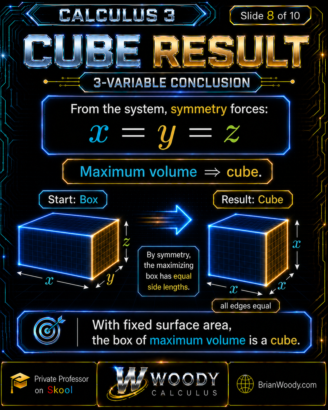
Why the Maximum-Volume Box Is a Cube
The three Lagrange equations force all three positive side lengths to be equal.
Because \(x\), \(y\), and \(z\) are positive, the divisions used below are valid.
From the first two multiplier equations:
\frac{yz}{2(y+z)}
=
\frac{xz}{2(x+z)}.
\]
Since \(z>0\):
\frac{y}{y+z}
=
\frac{x}{x+z}.
\]
Cross-multiply:
y(x+z)=x(y+z).
\]
xy+yz=xy+xz.
\]
Thus:
yz=xz
\quad\Longrightarrow\quad
y=x.
\]
Comparing another pair of equations similarly gives:
\boxed{x=y=z.}
\]
Use the Surface-Area Constraint
Let:
x=y=z=a.
\]
Then:
2a^2+2a^2+2a^2=S,
\]
6a^2=S.
\]
Since the side length is positive:
\boxed{
a=\sqrt{\frac{S}{6}}.
}
\]
Therefore:
\boxed{
x=y=z=\sqrt{\frac{S}{6}}.
}
\]
Find the Maximum Volume
\boxed{
V_{\max}
=
\left(\sqrt{\frac{S}{6}}\right)^3
=
\left(\frac{S}{6}\right)^{3/2}.
}
\]
Plain-language answer: with fixed surface area \(S\), the maximum-volume rectangular box is a cube with side length \(\sqrt{S/6}\) and volume \((S/6)^{3/2}\).
Additional Exam Example: Optimize \(f(x,y)=x+y\) on the Unit Circle
This example shows why every Lagrange candidate must be evaluated before deciding which point is the maximum or minimum.
Optimize:
f(x,y)=x+y
\]
subject to:
x^2+y^2=1.
\]
Step 1: Compute the Gradients
\nabla f=\langle1,1\rangle.
\]
\nabla g=\langle2x,2y\rangle.
\]
Step 2: Check the Constraint Qualification
The constraint gradient is zero only at:
(x,y)=(0,0).
\]
The origin is not on the unit circle, so every feasible point satisfies \(\nabla g\ne0\). The standard Lagrange multiplier theorem applies everywhere on the constraint.
Step 3: Set \(\nabla f=\lambda\nabla g\)
1=2\lambda x,
\qquad
1=2\lambda y.
\]
The equation \(1=2\lambda x\) forces \(\lambda\ne0\). Therefore:
x=\frac{1}{2\lambda}=y.
\]
Hence:
x=y.
\]
Step 4: Use the Constraint
2x^2=1.
\]
The candidates are:
\left(
\frac{1}{\sqrt2},
\frac{1}{\sqrt2}
\right),
\qquad
\left(
-\frac{1}{\sqrt2},
-\frac{1}{\sqrt2}
\right).
\]
Step 5: Evaluate the Objective
\boxed{
f_{\max}=\sqrt2,
\qquad
f_{\min}=-\sqrt2.
}
\]
Plain-language answer: the unit-circle maximum occurs in the direction \(\langle1,1\rangle\), while the minimum occurs in the opposite direction.
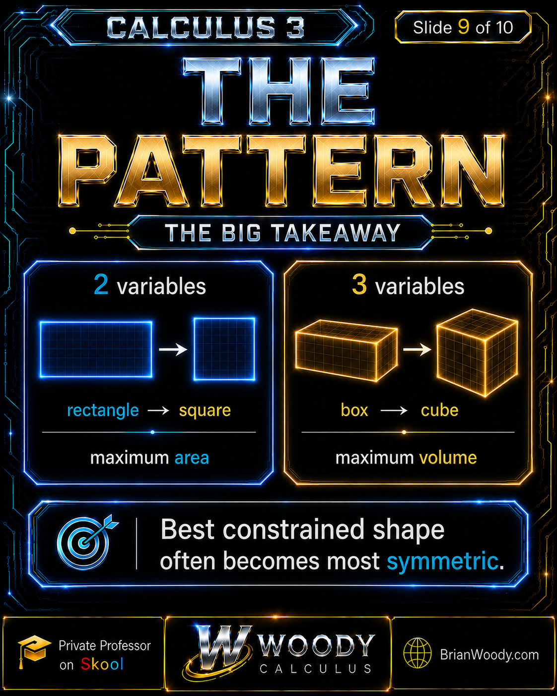
Why Does Symmetry Appear in Constrained Optimization?
When the objective and constraint treat the variables symmetrically, the optimizing point often has equal coordinates.
In the rectangle problem:
\text{rectangle}
\longrightarrow
\text{square}.
\]
In the box problem:
\text{rectangular box}
\longrightarrow
\text{cube}.
\]
This does not mean that every optimization problem produces equal variables. It means that symmetric data often produce symmetric critical points.
Lagrange multipliers make that hidden symmetry visible through the component equations.
What Does the Multiplier \(\lambda\) Mean?
At the candidate point, \(\lambda\) is the scalar that relates the objective gradient to the constraint gradient.
\nabla f=\lambda\nabla g.
\]
- If \(\lambda>0\), the gradients point in the same direction.
- If \(\lambda<0\), the gradients point in opposite directions.
- If \(\lambda=0\), then \(\nabla f=0\) at that candidate.
- The magnitude \(|\lambda|\) compares the sizes of the two gradients.
With the convention:
\mathcal{L}
=
f-\lambda(g-c),
\]
and under suitable regularity conditions, \(\lambda\) can also describe how the optimal objective value changes when the constraint value \(c\) changes slightly. This interpretation is often called a sensitivity value or shadow price.
Substitution vs. Lagrange Multipliers
Substitution reduces the number of variables, while Lagrange multipliers preserve the geometry and symmetry of the original problem.
| Method | Main Advantage | Main Limitation |
|---|---|---|
| Substitution | Can reduce a two-variable problem to ordinary single-variable calculus | May create complicated algebra or hide symmetry |
| Lagrange multipliers | Works directly with the objective and constraint gradients | Produces a simultaneous system that may be algebraically challenging |
If a constraint solves cleanly for one variable, substitution may be efficient. If the constraint is symmetric, implicit, or naturally geometric, Lagrange multipliers are often the better method.
How Do You Check and Classify Lagrange Multiplier Candidates?
Evaluate the objective function at every candidate and compare the resulting values.
A complete constrained-optimization analysis should consider:
- all solutions of \(\nabla f=\lambda\nabla g\),
- all feasible points where \(\nabla g=0\),
- endpoints, corners, or additional boundary components,
- the behavior of \(f\) if the constraint is unbounded.
If \(f\) is continuous and the constrained set is closed and bounded, the
Extreme Value Theorem
guarantees that global maximum and minimum values exist.
If the constraint is not compact, the objective may fail to attain a global extremum even when Lagrange candidates exist.
Lagrange Multipliers with Multiple Constraints
With two independent equality constraints, the objective gradient lies in the span of the two constraint gradients.
To optimize \(f(x,y,z)\) subject to:
g(x,y,z)=c,
\qquad
h(x,y,z)=d,
\]
solve:
\boxed{
\nabla f
=
\lambda\nabla g
+
\mu\nabla h.
}
\]
The complete system includes both original constraints.
Geometrically, the allowed motion lies along the intersection of the two constraint surfaces. Both constraint gradients are normal to the allowable tangent direction.
Common Lagrange Multiplier Mistakes
Mistake 1: Forgetting the Original Constraint
The gradient equations alone are incomplete. Always include \(g=c\).
Mistake 2: Setting \(\nabla f=\nabla g\)
The gradients need not have equal magnitude. Use \(\nabla f=\lambda\nabla g\).
Mistake 3: Assuming Parallel Means the Same Direction
A negative multiplier means the gradients point in opposite directions.
Mistake 4: Treating Every Candidate as a Maximum
Lagrange equations generate candidates. Compare the objective values.
Mistake 5: Ignoring Singular Constraint Points
If \(\nabla g=0\), check that feasible constraint point separately.
Mistake 6: Ignoring Endpoints or Corners
A constrained arc, segment, or piecewise boundary may have endpoints not captured by the regular equations.
Mistake 7: Using the Wrong Constraint Function
Write the constraint carefully and verify that its level set describes the intended feasible points.
Mistake 8: Losing Positivity Conditions
Lengths, areas, and physical dimensions may require \(x>0\), \(y>0\), and \(z>0\).
Mistake 9: Solving Components but Never Substituting Back
Use the original constraint to determine the actual coordinate values.
Mistake 10: Stopping at \(x=y\) or \(x=y=z\)
The symmetry relation is not the final answer. Use the constraint to find the dimensions and objective value.
The Woody Calculus Lagrange Multiplier Checklist
- State what is being maximized or minimized.
- Define the objective function \(f\).
- Write the constraint as \(g=c\).
- Record physical and domain restrictions.
- Compute \(\nabla f\) carefully.
- Compute \(\nabla g\) carefully.
- Set \(\nabla f=\lambda\nabla g\).
- Match corresponding components.
- Include the original constraint.
- Use symmetry before doing unnecessary algebra.
- Solve for every candidate.
- Check feasible singular points and boundaries.
- Evaluate the objective at every candidate.
- State the maximizing or minimizing point and value.
- Verify the result with geometry, symmetry, substitution, or an inequality when possible.
- Rewrite the complete solution from memory and say each step out loud.
Formula memorization is required, but the geometry controls the method: objective, constraint, gradients, system, candidates, comparison.
Lagrange Multipliers FAQ
What are Lagrange multipliers?
Lagrange multipliers are a method for optimizing a multivariable objective function while satisfying one or more equality constraints.
What is the Lagrange multiplier equation?
For an objective \(f\) and constraint \(g=c\), the central equation is \(\nabla f=\lambda\nabla g\), together with the original constraint.
Why do the gradients become parallel?
At a regular constrained extremum, both gradients are normal to the same tangent direction of the constraint. Therefore, they are scalar multiples.
Are the gradients always parallel in the same direction?
No. A positive multiplier gives the same direction, while a negative multiplier gives opposite directions.
Does solving the Lagrange equations automatically give a maximum?
No. The equations produce candidates. Evaluate the objective at every candidate and check singular points, endpoints, and boundaries.
What happens if the constraint gradient is zero?
The standard Lagrange multiplier theorem does not apply directly at a feasible point where \(\nabla g=0\). Check that point separately.
What does lambda mean in Lagrange multipliers?
The multiplier \(\lambda\) is the scalar relating the objective gradient to the constraint gradient. Under suitable conditions, it can also measure sensitivity to a change in the constraint value.
Can lambda be negative?
Yes. A negative multiplier means that the objective and constraint gradients point in opposite directions.
When should I use substitution instead?
Substitution may be simpler when the constraint solves cleanly for one variable. Lagrange multipliers are especially useful for symmetric or implicit constraints.
Why is the maximum-area rectangle a square?
For fixed perimeter \(P\), the Lagrange equations force \(x=y=P/4\), giving maximum area \(P^2/16\).
Why is the maximum-volume box a cube?
For fixed surface area \(S\), the multiplier equations force \(x=y=z=\sqrt{S/6}\), giving maximum volume \((S/6)^{3/2}\).
Can Lagrange multipliers handle two constraints?
Yes. With constraints \(g=c\) and \(h=d\), solve \(\nabla f=\lambda\nabla g+\mu\nabla h\) together with both constraints.
Master Lagrange Multipliers with Woody Calculus
Lagrange multipliers become manageable when students stop treating the method as a mysterious formula and start seeing the geometry.
The complete pattern is:
\text{objective}
\longrightarrow
\text{constraint}
\longrightarrow
\text{gradients}
\longrightarrow
\text{system}
\longrightarrow
\text{candidates}
\longrightarrow
\text{comparison}.
\]
For students who need structured support with gradients, partial derivatives, tangent planes, multiple integrals, vector fields, line integrals, Green’s Theorem, Stokes’ Theorem, and constrained optimization, begin in the
Woody Calculus Mastery Lab.
The Mastery Lab includes professor-led lessons, complete homework and exam solutions, live Q&A, direct chat support, practice exams, and the Woody Calculus problem-solving system.
Private Instruction
Brian M. Woody works privately with a limited number of serious students who need one-on-one help in
Calculus III,
Differential Equations,
Calculus II,
Abstract Algebra,
Real Analysis,
and advanced mathematics.
Private instruction is selective, requires weekly sessions, and requires enrollment in the
Woody Calculus Mastery Lab
first. Approval is not guaranteed.
Learn more through the
Private Math Tutor and Advanced Mathematics Instruction
page.
Related University Math Help Pages
Woody Calculus supports students at major universities with Calculus 3, multivariable calculus, Differential Equations, and advanced mathematics. Explore the complete
University Calculus Tutor Hub.
- Purdue Calculus 3 and Multivariable Optimization Help
- University of Florida Calculus 3 Support
- UCF Multivariable Calculus and Optimization Help
- Colorado State University Calculus 3 Help
- University of Nevada, Reno Multivariable Math Support
- Auburn Calculus 3 and Exam Preparation
- University of Alabama Calculus 3 Help
- University of Wisconsin Multivariable Calculus Tutor
- University of Michigan Calculus 3 Support
- UCLA Multivariable Calculus Help
- MIT Multivariable Calculus and Advanced Math Help
- Caltech Calculus 3 and Optimization Support
Trusted by Students Nationwide
Woody Calculus helps students build structure, confidence, and exam-ready mathematical skill in demanding STEM courses.
Read Woody Calculus 5-star Google reviews
and view Brian M. Woody’s
5.0 RateMyProfessors rating.