Calculus 3 • Multiple Integrals • Visual Lesson
Level: Undergraduate Calculus 3
|
Core skill: Translate a two-dimensional region into correct integration bounds
What Is a Double Integral?
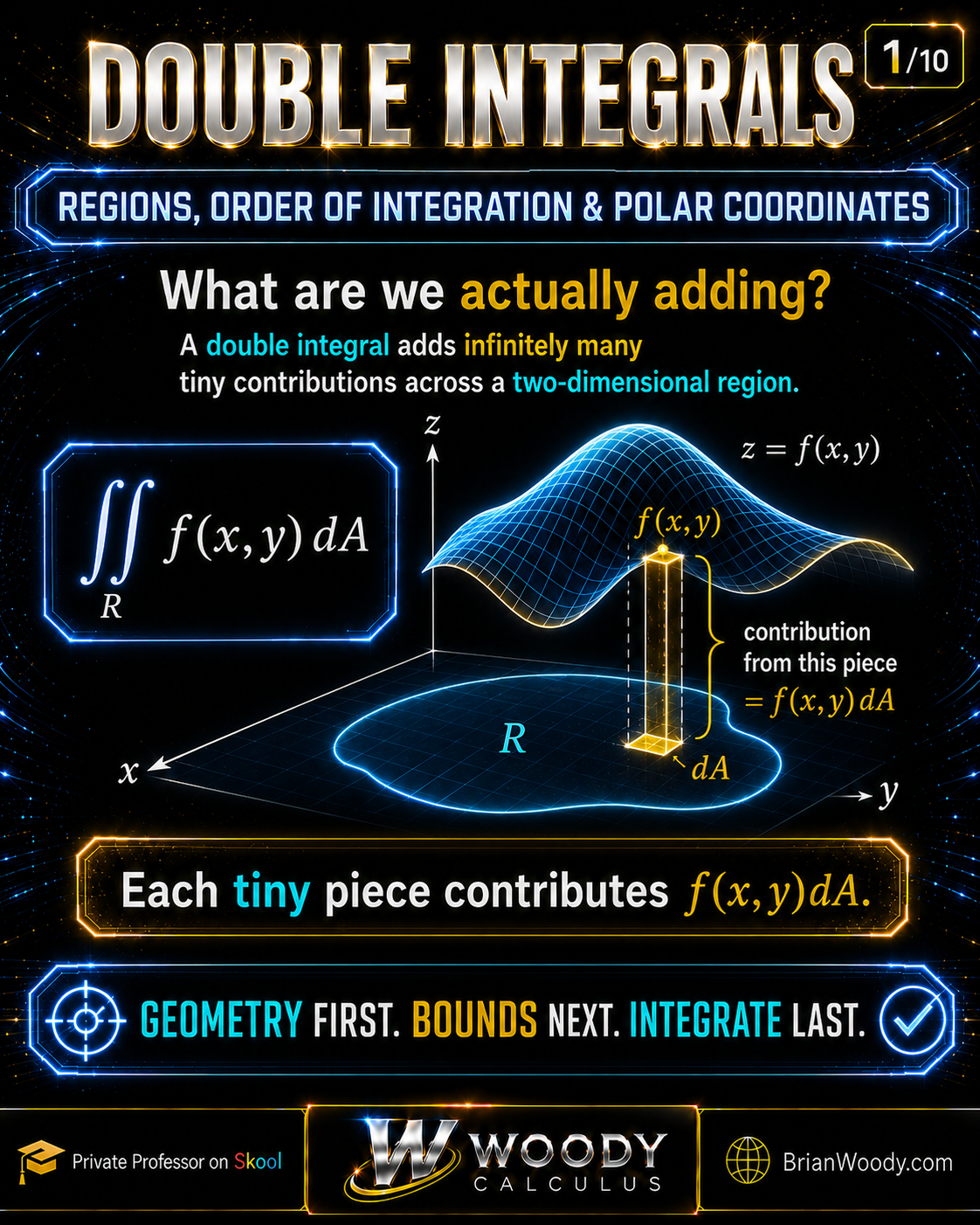
A double integral accumulates values of a function over a two-dimensional region.
The expression \(\iint_R f(x,y)\,dA\) adds infinitesimal contributions \(f(x,y)\,dA\)
across a region \(R\) in the \(xy\)-plane. If \(f\ge0\), it can represent volume under
\(z=f(x,y)\); if \(f=1\), it gives area; if \(f\) is a density, it can give mass.
Under the hypotheses of Fubini’s Theorem, we evaluate the double integral one variable at a time
as an iterated integral.
Geometry first. Bounds next. Integrate last.
Double Integrals: Key Takeaways
- A double integral accumulates infinitely many tiny contributions \(f(x,y)\,dA\) over a region.
- For continuous functions on rectangles, Fubini’s Theorem lets us evaluate the double integral in either iterated order.
- Type I regions use vertical slices and naturally lead to \(dy\,dx\).
- Type II regions use horizontal slices and naturally lead to \(dx\,dy\).
- Changing the order means redescribing the same geometric region—not merely swapping differentials.
- Polar coordinates are often the best choice for disks, annuli, sectors, and radial symmetry.
- The extra \(r\) in \(dA=r\,dr\,d\theta\) comes from geometry, not memorization.
Geometric Meaning of a Double Integral
A single integral adds contributions along a one-dimensional interval. A double integral does the
same basic job across a two-dimensional region. Imagine partitioning \(R\) into many tiny pieces
with areas \(\Delta A_{ij}\). Choose a sample point \((x_{ij}^*,y_{ij}^*)\) in each piece and form
\[
\sum_{i,j} f(x_{ij}^*,y_{ij}^*)\,\Delta A_{ij}.
\]
As the partition becomes finer, these Riemann sums approach the double integral when the appropriate
limit exists:
\[
\boxed{
\iint_R f(x,y)\,dA
=
\lim_{\|P\|\to0}
\sum_{i,j} f(x_{ij}^*,y_{ij}^*)\,\Delta A_{ij}
}.
\]
What does one tiny contribution mean?
If \(f(x,y)\ge0\), think of \(f(x,y)\) as a height above the point \((x,y)\).
A tiny base of area \(dA\) with height \(f(x,y)\) contributes approximately
\(f(x,y)\,dA\) units of volume. The double integral adds all of those tiny columns.
operator. Volume is one geometric interpretation when the integrand is nonnegative.
Rectangular Regions and Fubini’s Theorem
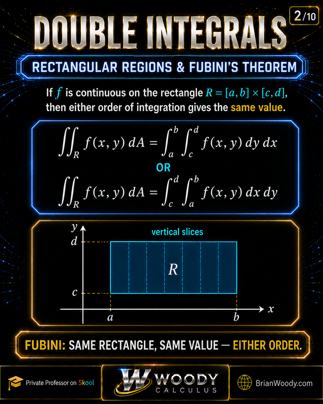
Suppose \(f\) is continuous on the rectangle
\[
R=[a,b]\times[c,d].
\]
Fubini’s Theorem allows us to evaluate the double integral by integrating one variable at a time:
\[
\boxed{
\iint_R f(x,y)\,dA
=
\int_a^b\!\int_c^d f(x,y)\,dy\,dx
=
\int_c^d\!\int_a^b f(x,y)\,dx\,dy
}.
\]
The continuity hypothesis is a clean Calc 3 condition guaranteeing the theorem applies on the rectangle.
Fubini’s Theorem has broader versions for integrable functions, but the continuous case captures the
central computational idea students use throughout multivariable calculus.
Worked rectangular example
Evaluate
\[
\int_0^2\!\int_1^3 (x+2y)\,dy\,dx.
\]
Integrate with respect to \(y\) first:
\[
\int_1^3(x+2y)\,dy
=
\left[xy+y^2\right]_1^3
=
2x+8.
\]
Then evaluate the outer integral:
\[
\int_0^2(2x+8)\,dx
=
\left[x^2+8x\right]_0^2
=
\boxed{20}.
\]
How Iterated Integrals Work

In the iterated integral
\[
\int_a^b
\left[
\int_c^d f(x,y)\,dy
\right]dx,
\]
the inner integral is performed first. During that inner integration, \(x\) behaves like a constant:
\[
I(x)=\int_c^d f(x,y)\,dy.
\]
The result is a function of \(x\). The outer integral then accumulates those slice values:
\[
\int_a^b I(x)\,dx.
\]
The differential written closest to the integrand tells you which variable is integrated first.
Type I Regions: Vertical Slices
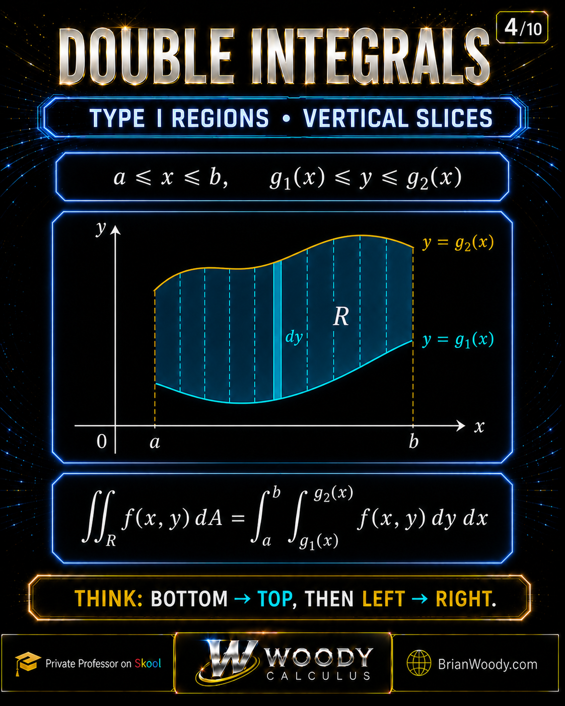
A Type I region is vertically simple. It can be described as
\[
\boxed{
a\le x\le b,
\qquad
g_1(x)\le y\le g_2(x)
}.
\]
For a fixed value of \(x\), move vertically through the region from the lower boundary
\(y=g_1(x)\) to the upper boundary \(y=g_2(x)\). Then let \(x\) sweep from \(a\) to \(b\):
\[
\boxed{
\iint_R f(x,y)\,dA
=
\int_a^b
\int_{g_1(x)}^{g_2(x)}
f(x,y)\,dy\,dx
}.
\]
A vertical slice is traversed in the \(y\)-direction, so \(dy\) is the inner differential.
The strip itself still has horizontal thickness \(dx\); the slide’s \(dy\) label identifies
the direction of inner integration.
Type I mental script: bottom → top, then left → right.
Type II Regions: Horizontal Slices
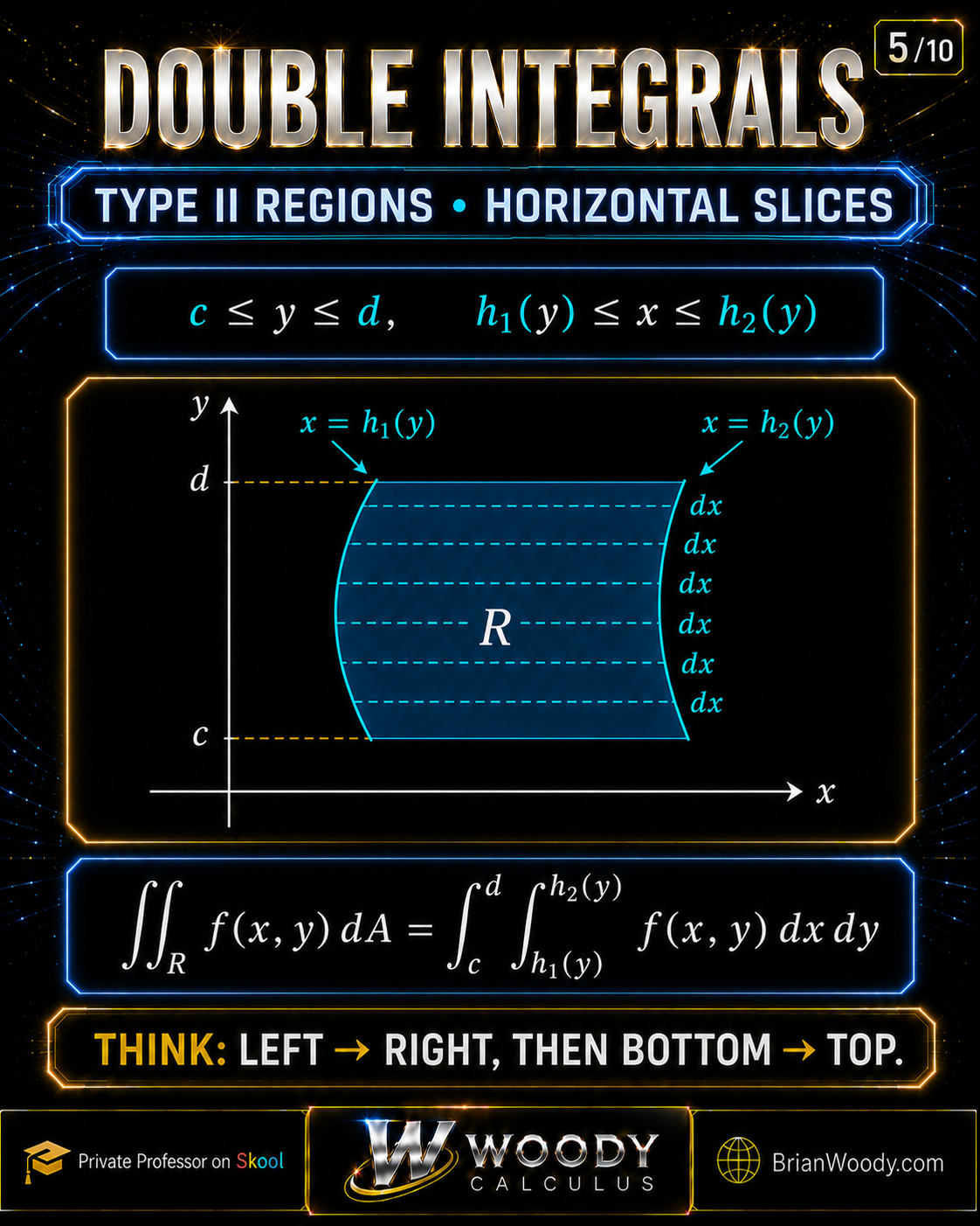
A Type II region is horizontally simple:
\[
\boxed{
c\le y\le d,
\qquad
h_1(y)\le x\le h_2(y)
}.
\]
For a fixed value of \(y\), move horizontally from the left boundary \(x=h_1(y)\)
to the right boundary \(x=h_2(y)\). Then sweep \(y\) from \(c\) to \(d\):
\[
\boxed{
\iint_R f(x,y)\,dA
=
\int_c^d
\int_{h_1(y)}^{h_2(y)}
f(x,y)\,dx\,dy
}.
\]
A horizontal slice is traversed in the \(x\)-direction, so \(dx\) is the inner differential.
The strip itself has vertical thickness \(dy\); the slide’s \(dx\) label identifies the direction
of inner integration.
Type II mental script: left → right, then bottom → top.
How Do You Choose the Order of Integration?
When both orders are possible, do not automatically choose \(dy\,dx\) just because it appears first
in a textbook. Choose the order that makes the region and integrand simpler.
| Question | Prefer \(dy\,dx\) | Prefer \(dx\,dy\) |
|---|---|---|
| Natural slices | Vertical slices are simple | Horizontal slices are simple |
| Boundary equations | Easy to solve for \(y\) | Easy to solve for \(x\) |
| Number of pieces | One Type I integral | One Type II integral |
| Antiderivative | Integrating in \(y\) first is easier | Integrating in \(x\) first is easier |
The Woody decision rule
- Draw the region. Identify every boundary curve.
- Try vertical slices. Can one slice move from one lower curve to one upper curve across the whole region?
- Try horizontal slices. Can one slice move from one left curve to one right curve across the whole region?
- Choose the cleaner description. Prefer fewer pieces and easier antiderivatives.
Changing the Order of Integration
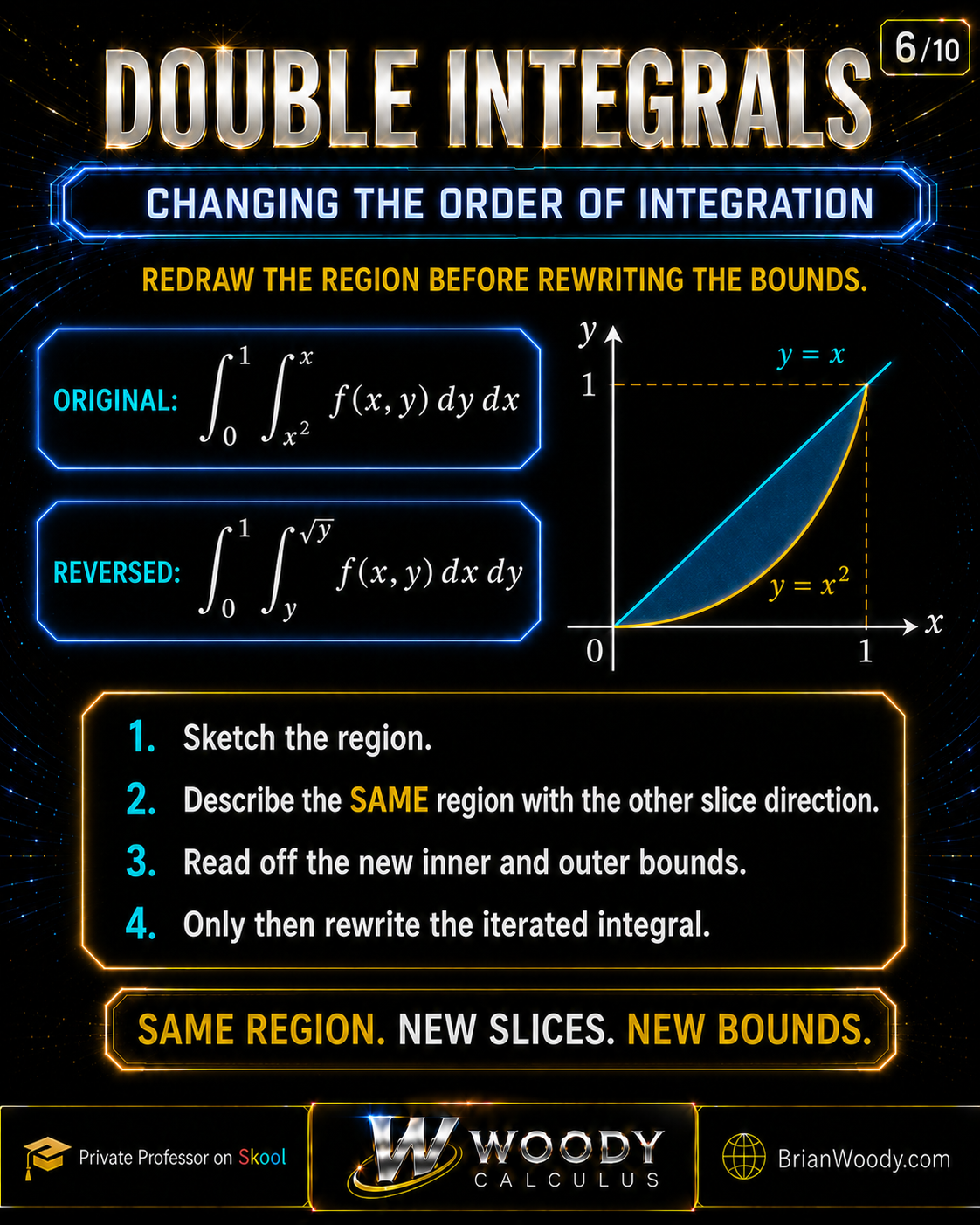
Consider the region described by
\[
0\le x\le1,
\qquad
x^2\le y\le x.
\]
The original Type I description is
\[
\boxed{
\int_0^1\int_{x^2}^{x}f(x,y)\,dy\,dx
}.
\]
To reverse the order, solve the boundary equations for \(x\):
\(y=x\) becomes \(x=y\), and \(y=x^2\) becomes \(x=\sqrt y\)
on the first-quadrant region. Horizontal slices therefore run from
\(x=y\) on the left to \(x=\sqrt y\) on the right, while
\(0\le y\le1\):
\[
\boxed{
\int_0^1\int_y^{\sqrt y}f(x,y)\,dx\,dy
}.
\]
Check the geometry by computing the area
Using vertical slices:
\[
A(R)
=
\int_0^1(x-x^2)\,dx
=
\frac12-\frac13
=
\boxed{\frac16}.
\]
Using horizontal slices:
\[
A(R)
=
\int_0^1(\sqrt y-y)\,dy
=
\frac23-\frac12
=
\boxed{\frac16}.
\]
Both descriptions produce the same area because they describe the same set of points.
This is a powerful sanity check when reversing integration order.
Applications of Double Integrals: Area, Volume, Mass, and Average Value
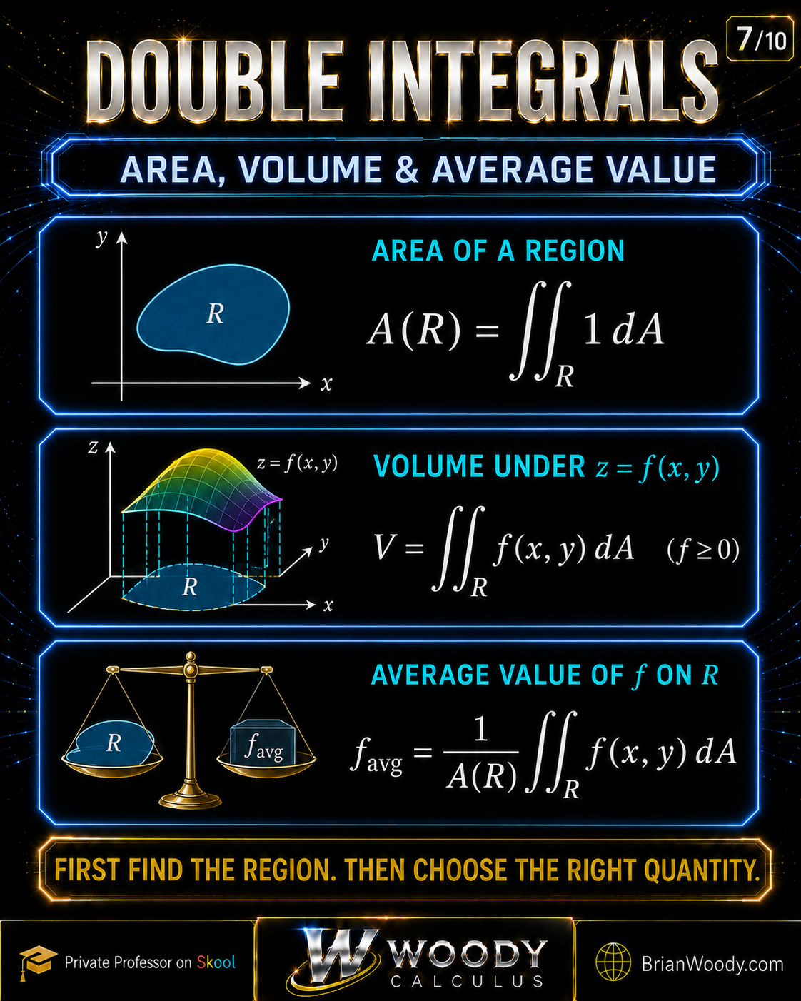
Area of a region
\[
\boxed{
A(R)=\iint_R1\,dA
}.
\]
Volume under a surface
If \(f(x,y)\ge0\) on \(R\), then
\[
\boxed{
V=\iint_R f(x,y)\,dA
}.
\]
If \(f\) takes both positive and negative values, the integral represents signed accumulation,
not ordinary geometric volume.
Mass from a density function
If \(\rho(x,y)\) is an areal density, then the total mass is
\[
\boxed{
M=\iint_R \rho(x,y)\,dA
}.
\]
Average value over a region
\[
\boxed{
f_{\mathrm{avg}}
=
\frac{1}{A(R)}
\iint_R f(x,y)\,dA
}.
\]
For example, on the unit square \(0\le x\le1\), \(0\le y\le1\),
the average value of \(f(x,y)=x+y\) is
\[
f_{\mathrm{avg}}
=
\int_0^1\!\int_0^1(x+y)\,dy\,dx
=
\boxed{1},
\]
because the area of the unit square is \(1\).
Double Integrals in Polar Coordinates
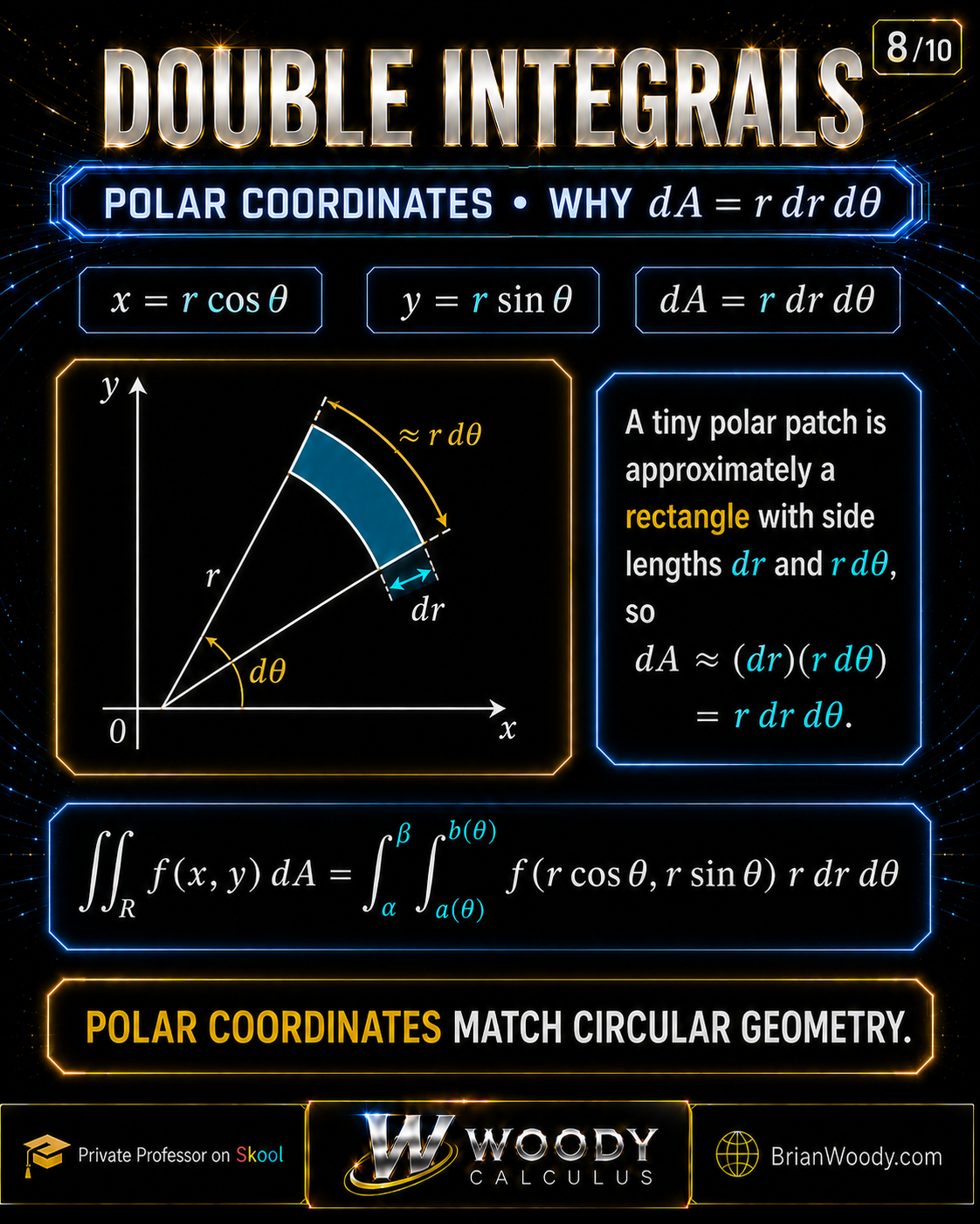
Cartesian coordinates are natural for rectangular geometry. Circular geometry often becomes
dramatically simpler in polar coordinates:
\[
x=r\cos\theta,
\qquad
y=r\sin\theta.
\]
Why is \(dA=r\,dr\,d\theta\)?
A tiny polar patch is not exactly a rectangle, but for very small \(dr\) and \(d\theta\)
it is approximately rectangular. Its radial side has length \(dr\), while its curved side has
approximate length \(r\,d\theta\). Therefore
\[
dA
\approx
(dr)(r\,d\theta)
=
r\,dr\,d\theta.
\]
This produces the polar double-integral formula
\[
\boxed{
\iint_R f(x,y)\,dA
=
\int_\alpha^\beta
\int_{a(\theta)}^{b(\theta)}
f(r\cos\theta,r\sin\theta)
\,r\,dr\,d\theta
}.
\]
Worked polar example
Evaluate \(\iint_R(x^2+y^2)\,dA\) over the unit disk.
Because \(x^2+y^2=r^2\) and \(dA=r\,dr\,d\theta\),
\[
\begin{aligned}
\iint_R(x^2+y^2)\,dA
&=
\int_0^{2\pi}\!\int_0^1 r^2(r)\,dr\,d\theta\\
&=
\int_0^{2\pi}
\left[\frac{r^4}{4}\right]_0^1
d\theta\\
&=
\frac14(2\pi)
=
\boxed{\frac\pi2}.
\end{aligned}
\]
The extra factor \(r\) is essential. Forgetting it changes the value of the integral.
One Region, Two Coordinate Systems: The Unit Disk
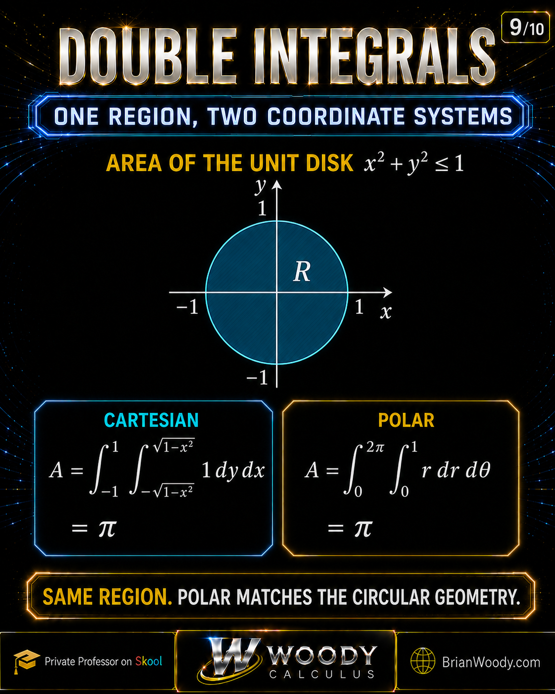
Let \(R\) be the unit disk
\[
R=\{(x,y):x^2+y^2\le1\}.
\]
Cartesian setup
\[
A(R)
=
\int_{-1}^1
\int_{-\sqrt{1-x^2}}^{\sqrt{1-x^2}}
1\,dy\,dx
=
\pi.
\]
Polar setup
\[
\begin{aligned}
A(R)
&=
\int_0^{2\pi}
\int_0^1
r\,dr\,d\theta\\
&=
\int_0^{2\pi}
\frac12\,d\theta
=
\boxed{\pi}.
\end{aligned}
\]
Both are correct. Polar coordinates are simply better aligned with the circular geometry.
Coordinate choice does not change the region or the answer—it changes the efficiency of the setup.
When a Region Must Be Split Into Multiple Integrals
Not every region can be described by one pair of inner boundaries for an entire outer interval.
Sometimes a vertical line or horizontal line enters the region through different boundary curves
depending on where the slice is located.
partway across the region, split the region at that transition point.
If \(R=R_1\cup R_2\) with disjoint interiors, then add the integrals:
\[
\boxed{
\iint_R f\,dA
=
\iint_{R_1}f\,dA
+
\iint_{R_2}f\,dA
}.
\]
This is another reason the picture comes before the antiderivative. The region decides the structure
of the integral.
What Comes After Double Integrals?
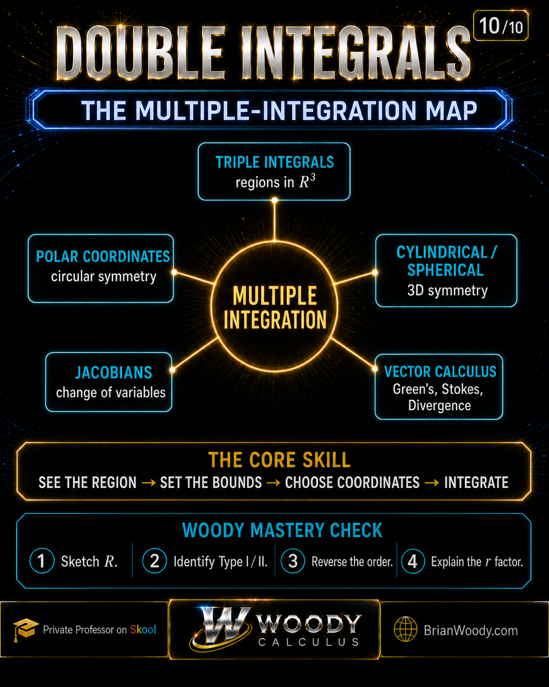
Double integrals are the gateway to the rest of multiple integration and vector calculus.
The same habits—visualize the region, choose coordinates, write bounds, then integrate—carry directly
into later Calculus 3 topics.
- Triple integrals: accumulation over three-dimensional regions.
- Cylindrical and spherical coordinates: coordinate systems matched to 3D symmetry.
- Jacobians: the general scaling factor behind changes of variables.
- Line and surface integrals: accumulation along curves and across surfaces.
- Green’s, Stokes’, and Divergence Theorems: deep relationships between local derivatives and global integrals.
Continue with
Jacobians and Change of Variables,
Cylindrical vs. Spherical Coordinates,
and
Green’s Theorem.
Common Double-Integral Mistakes
- Integrating before understanding the region. The bounds come from geometry.
- Mismatching the bounds and differentials. Inner bounds must match the inner variable.
- Swapping \(dx\) and \(dy\) without rewriting the bounds. Changing order requires a new description of the same region.
- Using the wrong boundary as left/right or bottom/top. Read one slice carefully.
- Forgetting that the outer bounds are constants in a simple Type I or Type II description.
- Forgetting to split a region when one boundary formula changes.
- Forgetting the factor \(r\) in polar coordinates.
- Using Cartesian coordinates for a circular region when polar would be dramatically simpler.
- Calling \(\iint_Rf\,dA\) geometric volume when \(f\) changes sign.
- Failing to check the answer against geometry. Area and ordinary volume should not be negative.
Woody Mastery Check
Close your notes and answer these aloud. The goal is not recognition—it is retrieval.
- Explain what \(\iint_R f(x,y)\,dA\) means geometrically.
- State the continuous-rectangle version of Fubini’s Theorem.
- Explain the difference between the inner and outer integrals.
- State the standard bounds for a Type I region.
- State the standard bounds for a Type II region.
- Explain why changing integration order requires redrawing the region.
- Reverse \(0\le x\le1\), \(x^2\le y\le x\).
- Explain why \(\iint_R1\,dA\) gives area.
- State the average-value formula over a region.
- Explain why \(dA=r\,dr\,d\theta\) in polar coordinates.
- Set up the area of the unit disk in both Cartesian and polar coordinates.
- Explain when a region must be split into multiple integrals.
Double Integrals FAQ
What is a double integral?
A double integral accumulates values of a function over a two-dimensional region. Depending on the integrand, it can represent signed accumulation, area, volume, mass, probability, or another total quantity.
What does dA mean in a double integral?
dA represents an infinitesimal area element in the plane. In Cartesian coordinates it is written as dy dx or dx dy when the double integral is evaluated as an iterated integral.
What is the geometric meaning of a double integral?
If f(x,y) is nonnegative, the double integral of f over R gives the volume under z=f(x,y) and above R. More generally, it measures signed accumulation of f across the region.
What is Fubini’s Theorem?
For a continuous function on a rectangular region, Fubini’s Theorem allows the double integral to be evaluated as an iterated integral in either order. Broader versions apply under more general integrability hypotheses.
What is an iterated integral?
An iterated integral evaluates a multiple integral one variable at a time. In a dy dx integral, integrate with respect to y first while x is treated as constant, then integrate the result with respect to x.
What is a Type I region?
A Type I region has x between two constants and y between a lower function and an upper function of x. It is naturally described using vertical slices and dy dx order.
What is a Type II region?
A Type II region has y between two constants and x between a left function and a right function of y. It is naturally described using horizontal slices and dx dy order.
How do you choose the bounds for a double integral?
Sketch the region first. Choose a slice direction, read the inner bounds along one slice, and then determine the outer interval over which those slices sweep through the region.
How do you change the order of integration?
Do not simply swap the differentials. Draw the region represented by the original bounds, choose the opposite slice direction, and rewrite both the inner and outer bounds so they describe the same region.
Why should you sketch the region before integrating?
The hardest part of many double-integral problems is translating geometry into correct bounds. A sketch shows the boundaries, the slice direction, and whether the region must be split into more than one integral.
Can every double integral be written in either order with one set of bounds?
No. Some regions are simple in one direction but require splitting into multiple pieces in the other direction. The geometry determines whether one iterated integral is enough.
How do double integrals find area?
Set the integrand equal to 1. Then the double integral of 1 over R adds the infinitesimal area elements dA and gives the total area A(R).
How do double integrals find volume?
If f(x,y) is nonnegative on R, the double integral of f over R gives the volume under the surface z=f(x,y) and above the region R.
How do you find the average value of a function over a region?
Divide the total accumulation by the area of the region: the average value equals one over A(R) times the double integral of f over R.
When should you use polar coordinates in a double integral?
Polar coordinates are especially effective when the region or integrand has circular or radial symmetry, such as disks, annuli, sectors, or expressions involving x squared plus y squared.
Why is there an r in dA = r dr dtheta?
A tiny polar patch has radial thickness dr and approximate arc length r dtheta. Multiplying those side lengths gives the area element r dr dtheta.
How do you integrate over the unit disk?
In Cartesian coordinates the unit disk uses square-root bounds. In polar coordinates it becomes 0 less than or equal to r less than or equal to 1 and 0 less than or equal to theta less than or equal to 2 pi, which is usually simpler.
What is the difference between Cartesian and polar double integrals?
Cartesian coordinates describe regions with x and y bounds and use dA=dx dy or dy dx. Polar coordinates use r and theta, replace x and y by r cos theta and r sin theta, and use dA=r dr dtheta.
What are the most common double-integral mistakes?
Common mistakes include skipping the region sketch, mismatching bounds and differentials, reversing the order by merely swapping symbols, forgetting the polar factor r, and using volume language when the integrand changes sign.
What topics come after double integrals in Calculus 3?
Double integrals lead naturally to triple integrals, cylindrical and spherical coordinates, Jacobians and change of variables, line and surface integrals, and Green’s, Stokes’, and Divergence Theorems.
References and Further Study
The definitions and standard theorem formulations in this lesson are consistent with established
multivariable-calculus treatments. For additional exercises and alternative presentations, see:
-
OpenStax Calculus Volume 3 — Double Integrals over Rectangular Regions
-
OpenStax Calculus Volume 3 — Double Integrals over General Regions
-
MIT OpenCourseWare — Double Integrals in Polar Coordinates
Related Woody Calculus Lessons
Need Help Mastering Double Integrals?
Double integrals are a major Calculus 3 turning point because geometry, algebra, and integration
must all work together. Train the process until it becomes automatic:
see the region → set the bounds → choose the coordinates → integrate.