Differential Equations • Second-Order Linear ODEs • Visual Lesson
Level: Undergraduate Differential Equations
|
Core skill: Find a particular solution when a forcing term does not fit the usual trial families
What Is Variation of Parameters?
Variation of Parameters is a systematic method for finding a particular solution of a nonhomogeneous linear differential equation.
If the homogeneous solution is \(y_h=C_1y_1+C_2y_2\), the method replaces the constants
\(C_1,C_2\) with functions \(u_1(t),u_2(t)\) and tries
\(y_p=u_1y_1+u_2y_2\). For
\(y^{\prime\prime}+p(t)y^{\prime}+q(t)y=r(t)\), the Wronskian formulas
\(u_1^{\prime}=-y_2r/W\) and \(u_2^{\prime}=y_1r/W\) determine those functions.
Core idea: replace constants with functions.
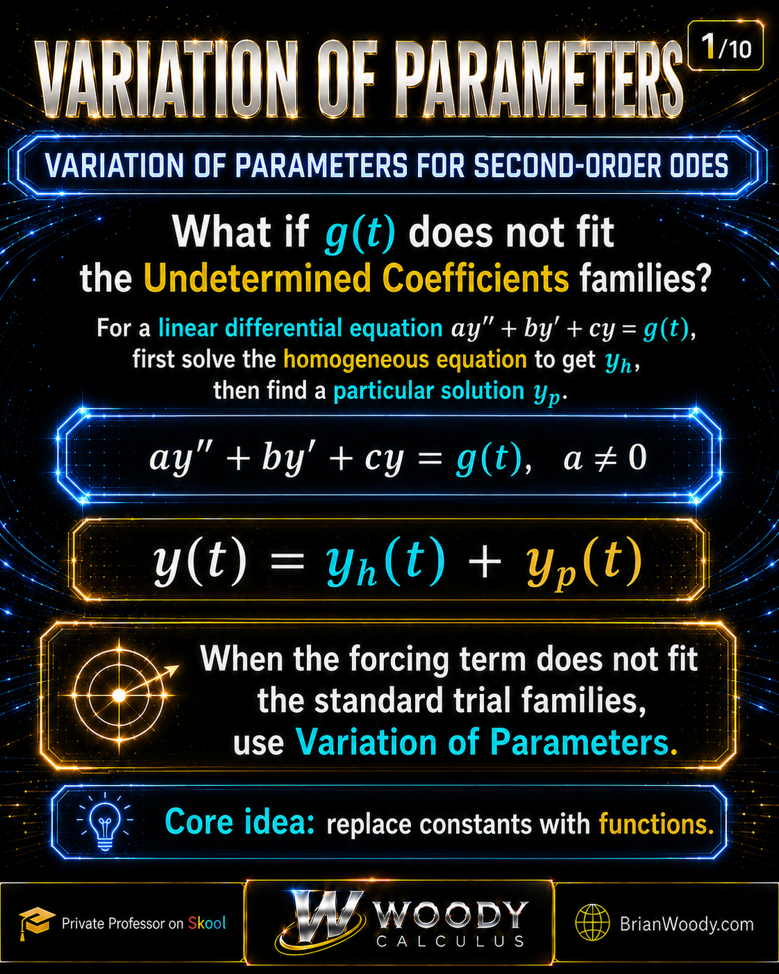
Variation of Parameters finds a particular solution by replacing constants with functions when the forcing term does not fit the usual Undetermined Coefficients families.
Variation of Parameters: Key Takeaways
- Always solve the associated homogeneous equation first.
- The method needs two linearly independent homogeneous solutions \(y_1,y_2\).
- Replace the homogeneous constants by functions: \(C_1,C_2\rightarrow u_1(t),u_2(t)\).
- Impose \(u_1^{\prime}y_1+u_2^{\prime}y_2=0\) to simplify the derivative algebra.
- Normalize the equation before using the memorized standard-form formulas.
- The Wronskian determines \(u_1^{\prime}\) and \(u_2^{\prime}\).
- Integration constants in \(u_1,u_2\) may be taken as zero because they only recreate homogeneous terms.
- Variation of Parameters can handle many forcing functions and variable-coefficient equations that Undetermined Coefficients cannot.
When Should You Use Variation of Parameters?
Consider a nonhomogeneous second-order linear differential equation
\[
ay^{\prime\prime}+by^{\prime}+cy=g(t),
\qquad a\ne0.
\]
The general solution has the familiar structure
\[
\boxed{y=y_h+y_p}.
\]
Undetermined Coefficients is usually the fastest method when the coefficients are constant and the
forcing term belongs to the standard polynomial, exponential, sine, cosine, or finite products of these.
Variation of Parameters does not require that kind of forcing-function guess. Instead, it uses the
known homogeneous solutions and integration.
Important nuance:
Variation of Parameters is not only a fallback.
It can also work when Undetermined Coefficients would work.
We normally choose Undetermined Coefficients in those cases because it is shorter.
The Woody Recognition Rule
Constant coefficients + forcing fits the UC families?
Try Undetermined Coefficients first.
Forcing does not fit, or coefficients vary, but \(y_1,y_2\) are known?
Variation of Parameters is a natural choice.
Step 1: Solve the Homogeneous Equation First
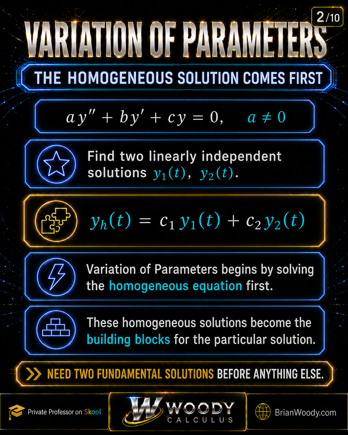
Solve the homogeneous equation first and find two linearly independent solutions y1 and y2; they become the building blocks for the particular solution.
For the normalized linear equation
\[
y^{\prime\prime}+p(t)y^{\prime}+q(t)y=r(t).
\]
First solve the associated homogeneous equation
\[
y^{\prime\prime}+p(t)y^{\prime}+q(t)y=0.
\]
Suppose \(y_1(t)\) and \(y_2(t)\) are two linearly independent solutions on an interval \(I\).
Then the homogeneous solution is
\[
\boxed{
y_h=C_1y_1+C_2y_2
}.
\]
These two functions are not a preliminary detail.
They are the actual building blocks used to construct the particular solution.
If the equation has constant coefficients, this is where the
characteristic equation
enters.
Step 2: Replace the Constants With Functions
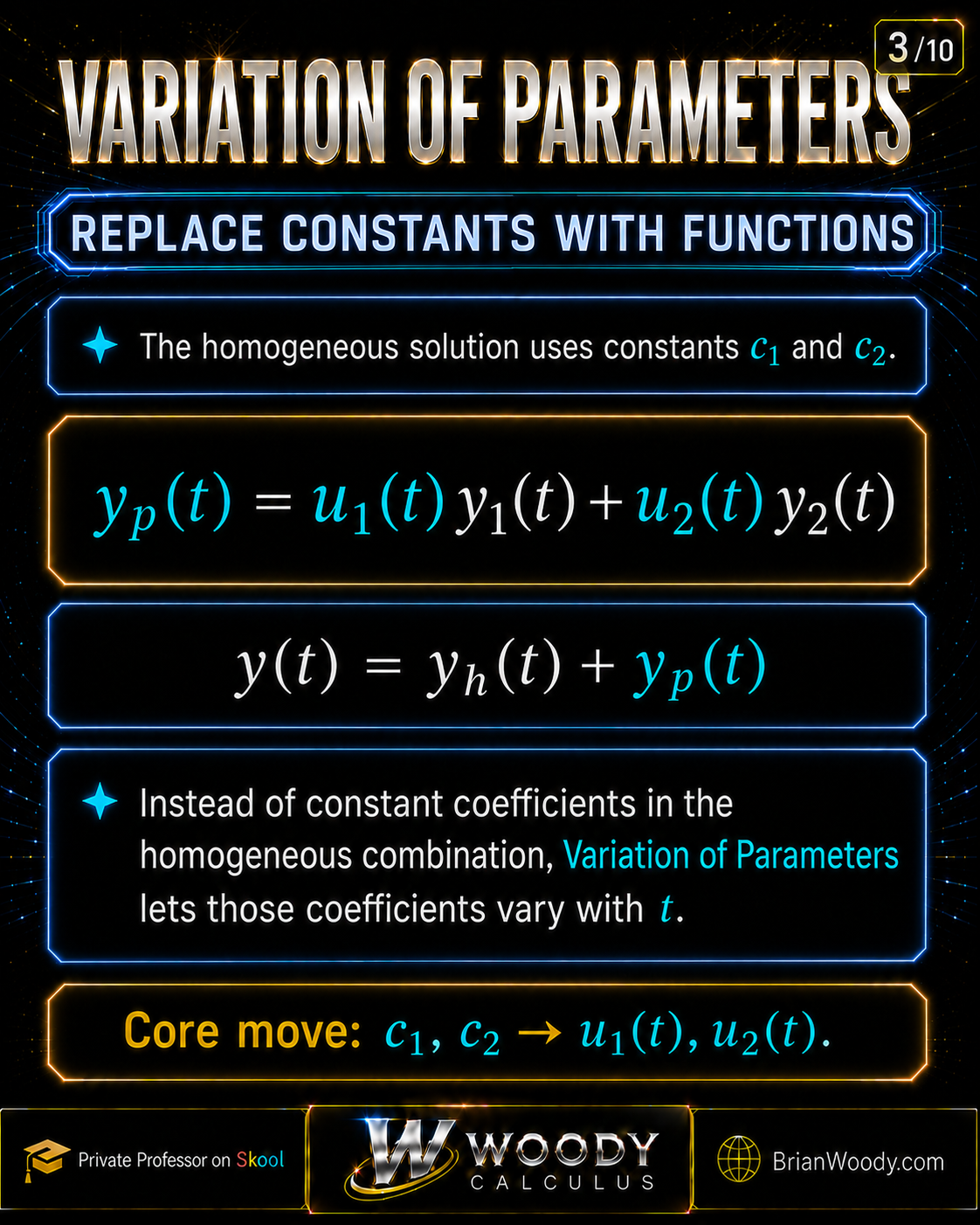
The core move in Variation of Parameters is to replace the homogeneous constants with functions u1(t) and u2(t).
The homogeneous solution uses constant coefficients \(C_1\) and \(C_2\).
Variation of Parameters allows those coefficients to vary with \(t\):
\[
C_1,C_2
\quad\longrightarrow\quad
u_1(t),u_2(t).
\]
We seek a particular solution of the form
\[
\boxed{
y_p=u_1y_1+u_2y_2
}.
\]
The idea is simple but powerful:
keep the same homogeneous basis \(y_1,y_2\), but let the coefficients flex with the forcing term \(r(t)\).
Step 3: Why Do We Impose the Auxiliary Condition?
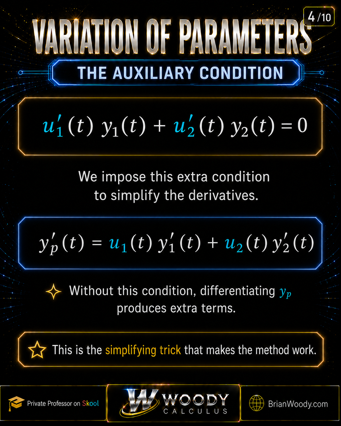
The auxiliary condition u1′ y1 + u2′ y2 = 0 is a chosen simplifying condition that removes extra derivative terms.
Differentiating
\(y_p=u_1y_1+u_2y_2\) gives
\[
y_p^{\prime}
=
u_1^{\prime}y_1+u_1y_1^{\prime}
+
u_2^{\prime}y_2+u_2y_2^{\prime}.
\]
We have two unknown functions \(u_1,u_2\), and the representation of \(y_p\) in this form has extra freedom.
We use that freedom to impose the simplifying condition
\[
\boxed{
u_1^{\prime}y_1+u_2^{\prime}y_2=0
}.
\]
The first derivative collapses to
\[
\boxed{
y_p^{\prime}=u_1y_1^{\prime}+u_2y_2^{\prime}
}.
\]
This condition is chosen, not discovered.
It is the simplifying choice that turns the method into a manageable two-equation linear system.
Step 4: Derive the Two-Equation System
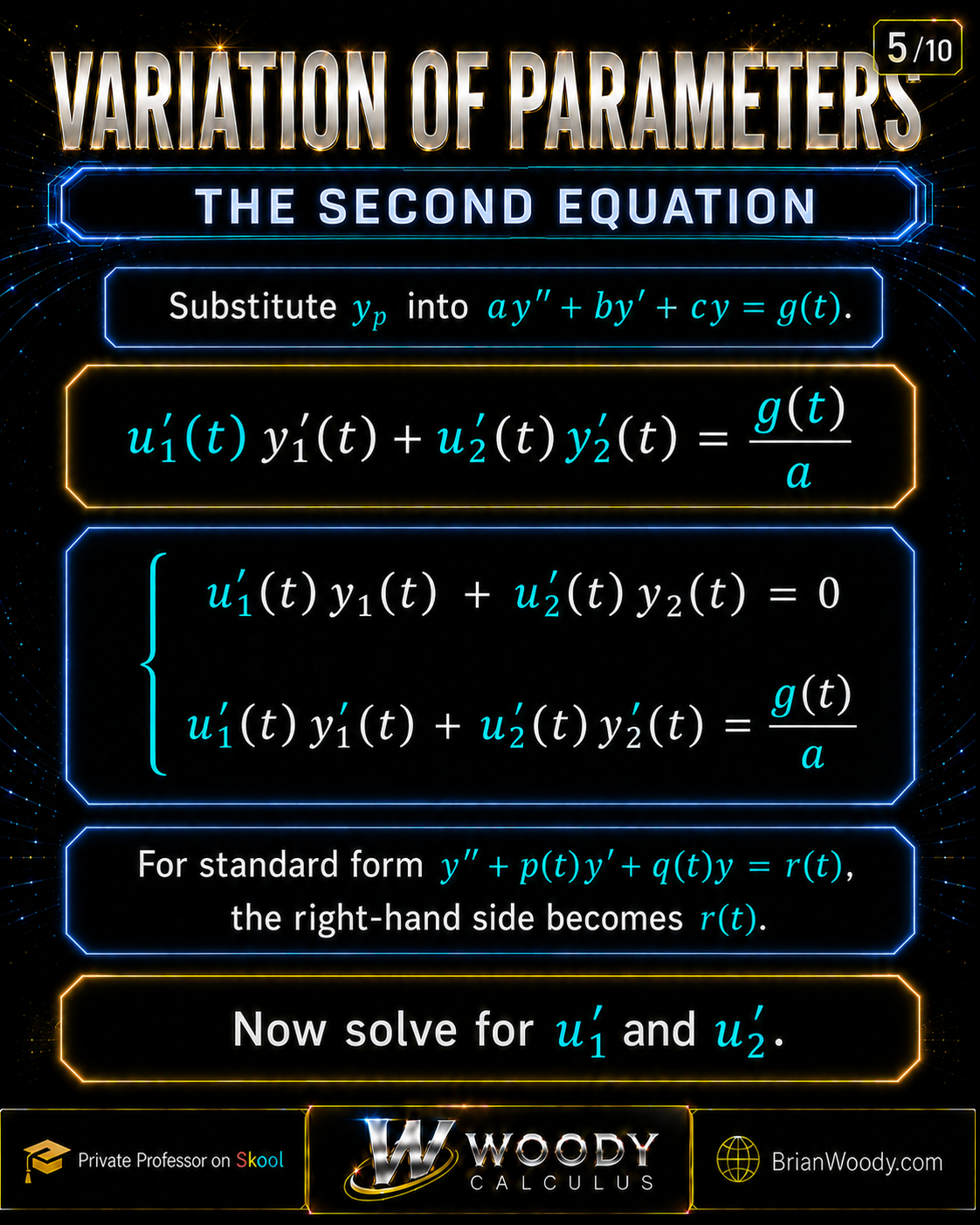
Substitution produces a two-by-two system for u1′ and u2′, including the critical factor g(t)/a before standardization.
Differentiate the simplified first derivative:
\[
y_p^{\prime\prime}
=
u_1^{\prime}y_1^{\prime}+u_2^{\prime}y_2^{\prime}
+
u_1y_1^{\prime\prime}+u_2y_2^{\prime\prime}.
\]
Substitute \(y_p,y_p^{\prime},y_p^{\prime\prime}\) into the normalized equation
\(y^{\prime\prime}+p(t)y^{\prime}+q(t)y=r(t)\):
\[
u_1^{\prime}y_1^{\prime}+u_2^{\prime}y_2^{\prime}
+
u_1\!\left(y_1^{\prime\prime}+py_1^{\prime}+qy_1\right)
+
u_2\!\left(y_2^{\prime\prime}+py_2^{\prime}+qy_2\right)
=
r(t).
\]
Since \(y_1,y_2\) solve the homogeneous equation, the bracketed terms vanish.
Therefore
\[
\boxed{
u_1^{\prime}y_1^{\prime}+u_2^{\prime}y_2^{\prime}=r(t)
}.
\]
Combined with the auxiliary condition, we obtain
\[
\boxed{
\begin{cases}
u_1^{\prime}y_1+u_2^{\prime}y_2=0,\\[4pt]
u_1^{\prime}y_1^{\prime}+u_2^{\prime}y_2^{\prime}=r(t).
\end{cases}
}
\]
The Leading-Coefficient Trap
If the original equation is
\[
ay^{\prime\prime}+by^{\prime}+cy=g(t),
\]
divide by \(a\) first.
Then \(r(t)=g(t)/a\), so the second equation in the system is
\[
\boxed{
u_1^{\prime}y_1^{\prime}+u_2^{\prime}y_2^{\prime}=\frac{g(t)}{a}
}.
\]
Step 5: Solve the System With the Wronskian
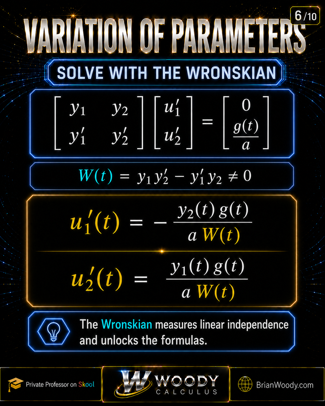
Cramer’s Rule and the Wronskian solve the two-equation system for u1′ and u2′.
The coefficient matrix of the two-equation system is
\[
\begin{bmatrix}
y_1 & y_2\\
y_1^{\prime} & y_2^{\prime}
\end{bmatrix}
\begin{bmatrix}
u_1^{\prime}\\
u_2^{\prime}
\end{bmatrix}
=
\begin{bmatrix}
0\\
r(t)
\end{bmatrix}.
\]
Its determinant is the Wronskian:
\[
\boxed{
W(t)
=
\begin{vmatrix}
y_1&y_2\\
y_1^{\prime}&y_2^{\prime}
\end{vmatrix}
=
y_1y_2^{\prime}-y_1^{\prime}y_2
}.
\]
For two linearly independent solutions of the same second-order linear homogeneous ODE on an interval,
\(W(t)\) does not vanish on that interval.
Solving the system with Cramer’s Rule gives
\[
\boxed{
u_1^{\prime}=-\frac{y_2r}{W},
\qquad
u_2^{\prime}=\frac{y_1r}{W}
}.
\]
For \(ay^{\prime\prime}+by^{\prime}+cy=g(t)\), these become
\[
\boxed{
u_1^{\prime}=-\frac{y_2g}{aW},
\qquad
u_2^{\prime}=\frac{y_1g}{aW}
}.
\]
Step 6: Integrate to Find \(u_1\), \(u_2\), and \(y_p\)
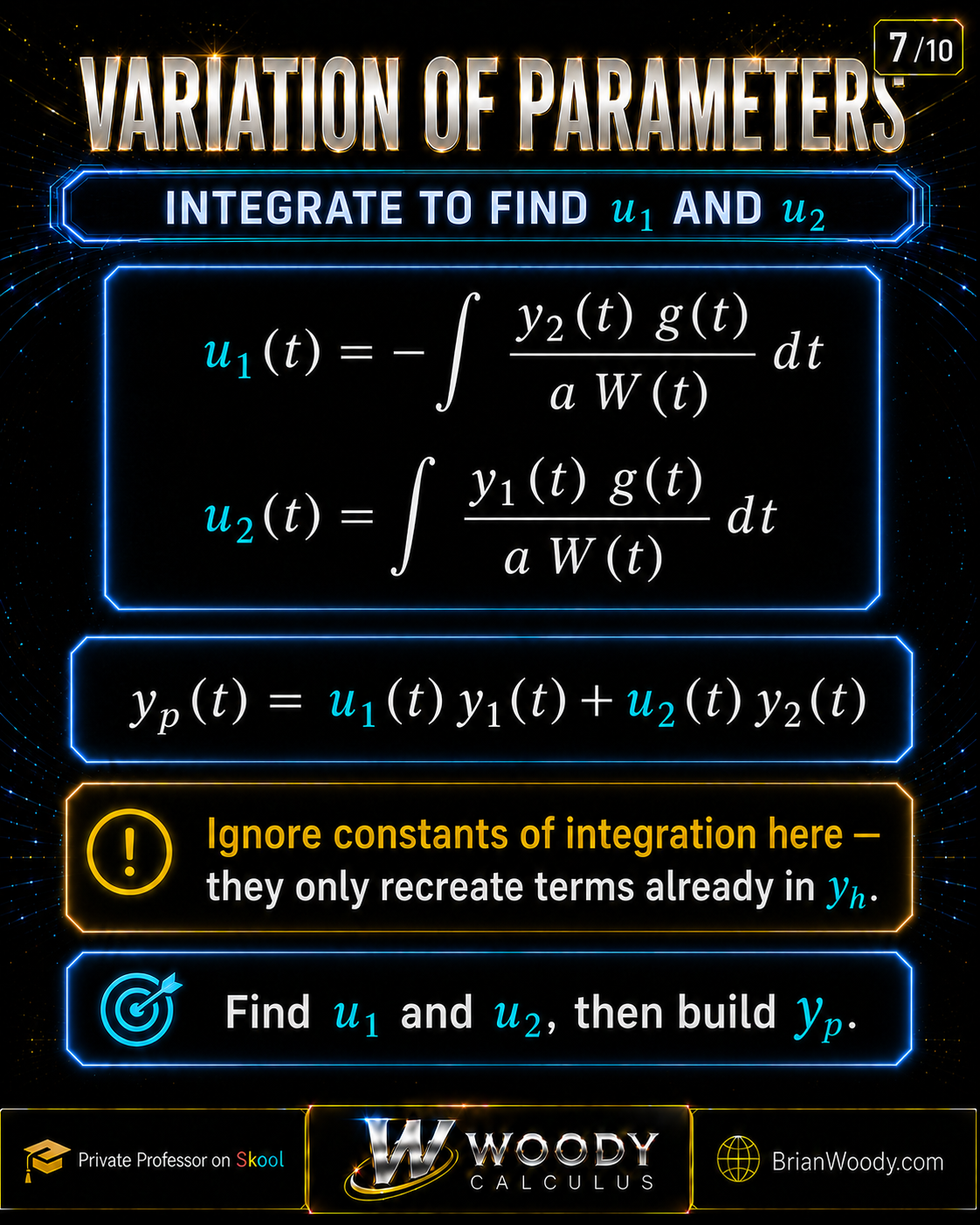
Integrate u1′ and u2′, ignore integration constants that only reproduce homogeneous terms, and build the particular solution.
Integrate the parameter derivatives:
\[
u_1
=
-\int\frac{y_2r}{W}\,dt,
\qquad
u_2
=
\int\frac{y_1r}{W}\,dt.
\]
Then substitute into \(y_p=u_1y_1+u_2y_2\):
\[
\boxed{
y_p
=
-y_1\int\frac{y_2r}{W}\,dt
+
y_2\int\frac{y_1r}{W}\,dt
}.
\]
Why Can We Ignore the Integration Constants?
Suppose the antiderivatives produce constants \(K_1,K_2\).
Then \(y_p\) changes by
\[
K_1y_1+K_2y_2,
\]
which is already part of the homogeneous solution \(y_h=C_1y_1+C_2y_2\).
Therefore we may choose the integration constants in \(u_1,u_2\) to be zero without losing any solutions.
The Standard-Form Variation of Parameters Formula
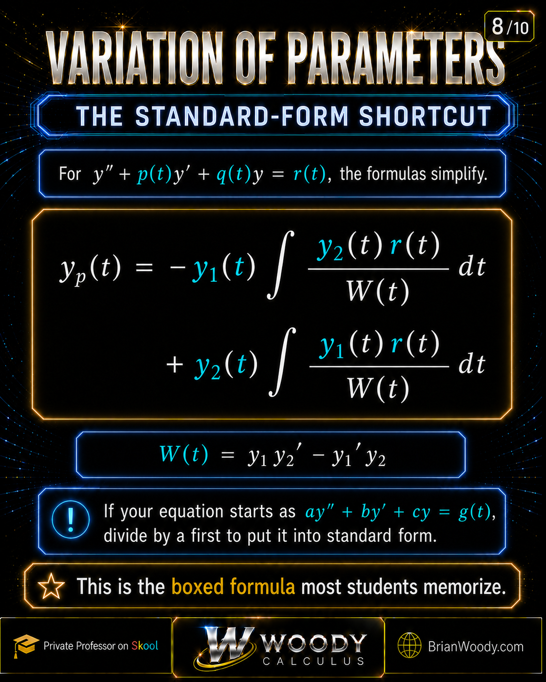
In standard form, the leading coefficient is 1 and the Variation of Parameters formula simplifies to the familiar Wronskian shortcut.
For
\[
y^{\prime\prime}+p(t)y^{\prime}+q(t)y=r(t),
\]
the formula most students memorize is
\[
\boxed{
y_p(t)
=
-y_1(t)\int\frac{y_2(t)r(t)}{W(t)}\,dt
+
y_2(t)\int\frac{y_1(t)r(t)}{W(t)}\,dt
}.
\]
Do not use this formula on an unnormalized equation.
If the coefficient of \(y^{\prime\prime}\) is not \(1\), divide the entire differential equation by that coefficient first.
Worked Example: Solve \(y^{\prime\prime}+y=\sec t\)
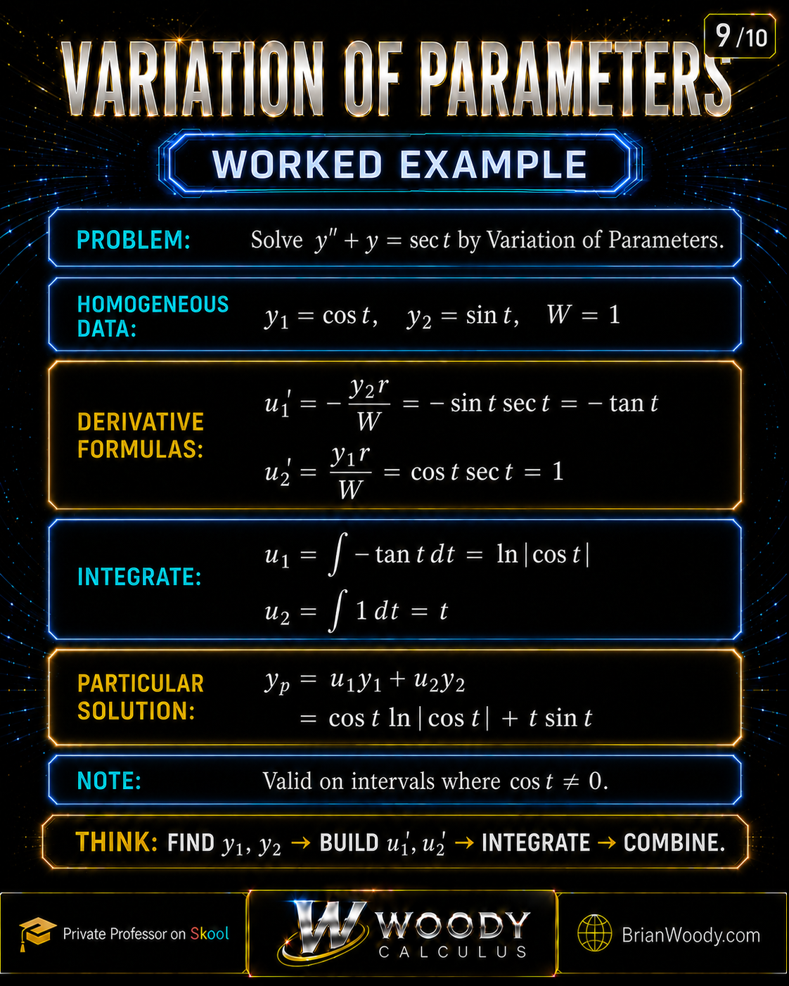
Solving y”+y=sec t gives yp=cos(t) ln|cos t|+t sin t on intervals where cos t is nonzero.
This example is ideal for Variation of Parameters because \(\sec t\) is not one of the standard
Undetermined Coefficients forcing families.
Work on any interval where \(\cos t\ne0\).
1. Solve the Homogeneous Equation
\[
y^{\prime\prime}+y=0.
\]
The characteristic equation is \(m^2+1=0\), so choose
\[
y_1=\cos t,
\qquad
y_2=\sin t.
\]
2. Compute the Wronskian
\[
W
=
\begin{vmatrix}
\cos t&\sin t\\
-\sin t&\cos t
\end{vmatrix}
=
\cos^2t+\sin^2t
=
\boxed{1}.
\]
3. Find \(u_1^{\prime}\) and \(u_2^{\prime}\)
Here \(r(t)=\sec t\).
Therefore
\[
u_1^{\prime}
=
-\frac{(\sin t)(\sec t)}{1}
=
-\tan t,
\qquad
u_2^{\prime}
=
\frac{(\cos t)(\sec t)}{1}
=
1.
\]
4. Integrate
\[
u_1
=
\int-\tan t\,dt
=
\ln|\cos t|,
\qquad
u_2
=
\int1\,dt
=
t.
\]
5. Build the Particular Solution
\[
\boxed{
y_p
=
\cos t\,\ln|\cos t|
+
t\sin t
}.
\]
The general solution on the chosen interval is
\[
\boxed{
y
=
C_1\cos t
+
C_2\sin t
+
\cos t\,\ln|\cos t|
+
t\sin t
}.
\]
Verify the Particular Solution
A high-value habit in Differential Equations is to verify a complicated particular solution.
Start with
\[
y_p=\cos t\,\ln|\cos t|+t\sin t.
\]
Differentiate. After the \(-\sin t\) and \(+\sin t\) terms cancel, the simplified derivative is
\[
y_p^{\prime}
=
-\sin t\,\ln|\cos t|
+
t\cos t.
\]
Differentiating again gives
\[
y_p^{\prime\prime}
=
-\cos t\,\ln|\cos t|
+
\sin t\tan t
+
\cos t
–
t\sin t.
\]
Therefore
\[
\begin{aligned}
y_p^{\prime\prime}+y_p
&=
\sin t\tan t+\cos t\\
&=
\frac{\sin^2t}{\cos t}+\cos t\\
&=
\frac{\sin^2t+\cos^2t}{\cos t}\\
&=
\boxed{\sec t}.
\end{aligned}
\]
Verification passed.
This is not busywork: it catches sign errors in \(u_1^{\prime}\), \(u_2^{\prime}\), and the Wronskian formula.
Bonus: Variation of Parameters With Variable Coefficients
One reason Variation of Parameters is more general than Undetermined Coefficients is that the
coefficients of the differential equation may vary with \(t\), provided a fundamental pair
\(y_1,y_2\) is known.
Consider, for \(t\gt0\),
\[
y^{\prime\prime}
–
\frac{2}{t}y^{\prime}
+
\frac{2}{t^2}y
=
t.
\]
The homogeneous equation has the linearly independent solutions
\[
y_1=t,
\qquad
y_2=t^2.
\]
The Wronskian is
\[
W
=
t(2t)-(1)(t^2)
=
t^2.
\]
With \(r(t)=t\),
\[
u_1^{\prime}
=
-\frac{t^2(t)}{t^2}
=
-t,
\qquad
u_2^{\prime}
=
\frac{t(t)}{t^2}
=
1.
\]
Choose
\[
u_1=-\frac{t^2}{2},
\qquad
u_2=t.
\]
Then
\[
\boxed{
y_p
=
u_1y_1+u_2y_2
=
-\frac{t^3}{2}+t^3
=
\frac{t^3}{2}
}.
\]
Substitution confirms that this \(y_p\) produces the forcing term \(t\).
This example shows why Variation of Parameters is not limited to constant-coefficient ODEs.
Undetermined Coefficients vs. Variation of Parameters
| Feature | Undetermined Coefficients | Variation of Parameters |
|---|---|---|
| Forcing term | Special polynomial/exponential/trigonometric families and finite combinations | Many forcing functions, including functions outside those trial families |
| Coefficients | Usually constant coefficients | Can handle variable coefficients if \(y_1,y_2\) are known |
| Main idea | Guess the form of \(y_p\) | Replace homogeneous constants with functions |
| Computation | Mostly algebra | Wronskian formulas plus integration |
| Speed | Usually faster when applicable | Usually longer but more general |
Continue with the companion lesson
Undetermined Coefficients: Particular Solutions
to compare the methods directly.
Which Differential-Equations Method Should You Choose?
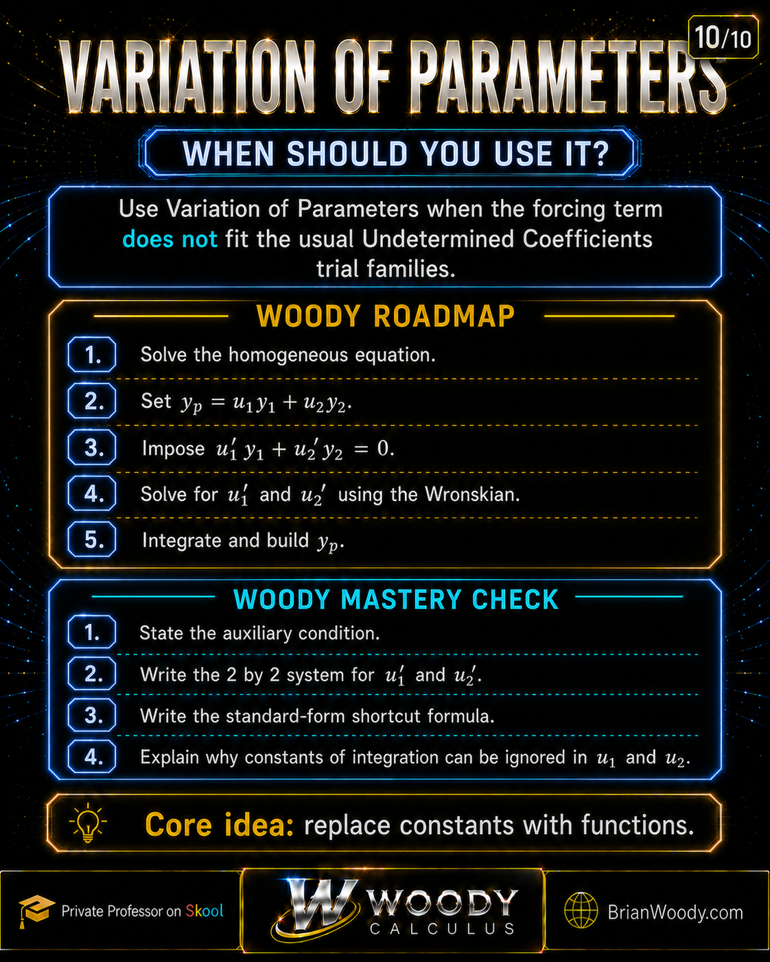
The Woody Roadmap summarizes the full Variation of Parameters algorithm and when to choose it.
Homogeneous Equation
Start with the characteristic equation when coefficients are constant.
Undetermined Coefficients
Use when the forcing term belongs to a recognized trial family and the coefficients are constant.
Variation of Parameters
Use when homogeneous solutions are known and you need a systematic particular-solution method.
Laplace Transforms
Especially useful for initial-value problems, piecewise forcing, and impulse inputs.
Power Series
Useful when coefficient functions prevent elementary closed-form homogeneous solutions.
Exam-Day Recognition
Do not start integrating until you have identified the method.
Recognize the equation type, normalize it, solve the homogeneous problem, inspect the forcing term,
and then choose the shortest valid method.
Common Variation of Parameters Mistakes
- Forgetting to normalize the equation. The shortcut formulas assume the coefficient of \(y^{\prime\prime}\) is \(1\).
- Using the wrong sign in \(u_1^{\prime}\). The first formula carries the minus sign.
- Computing the Wronskian backwards. Use \(W=y_1y_2^{\prime}-y_1^{\prime}y_2\).
- Skipping the homogeneous solution. Variation of Parameters cannot begin until \(y_1,y_2\) are known.
- Forgetting the auxiliary condition. It is what reduces the derivative algebra to a solvable system.
- Adding unnecessary constants to \(u_1,u_2\). Those constants are absorbed into \(y_h\).
- Forgetting the domain of the forcing term. A forcing function such as \(\sec t\) restricts the interval of validity.
- Assuming Variation of Parameters only works for constant coefficients. It works more generally when a fundamental homogeneous set is known.
- Using Variation of Parameters when a much shorter method is obvious. Generality does not always mean efficiency.
- Failing to verify a complicated particular solution. A direct substitution can expose a sign or integration error immediately.
Variation of Parameters Quick Reference
Standard Form
\[
y^{\prime\prime}+p(t)y^{\prime}+q(t)y=r(t).
\]
Homogeneous Basis
\[
y_h=C_1y_1+C_2y_2.
\]
Particular-Solution Form
\[
y_p=u_1y_1+u_2y_2.
\]
Wronskian
\[
W=y_1y_2^{\prime}-y_1^{\prime}y_2.
\]
Parameter Derivatives
\[
u_1^{\prime}=-\frac{y_2r}{W},
\qquad
u_2^{\prime}=\frac{y_1r}{W}.
\]
Particular Solution
\[
\boxed{
y_p
=
-y_1\int\frac{y_2r}{W}\,dt
+
y_2\int\frac{y_1r}{W}\,dt
}.
\]
- Normalize: Divide by the leading coefficient so the coefficient of \(y^{\prime\prime}\) is \(1\).
- Solve the homogeneous equation: Find two linearly independent solutions \(y_1\) and \(y_2\).
- Vary the constants: Set \(y_p=u_1y_1+u_2y_2\).
- Impose the auxiliary condition: Use \(u_1^{\prime}y_1+u_2^{\prime}y_2=0\).
- Compute the Wronskian formulas: Find \(W\), then compute \(u_1^{\prime}\) and \(u_2^{\prime}\).
- Integrate: Find \(u_1\) and \(u_2\), taking unnecessary integration constants to be zero.
- Assemble the solution: Build \(y_p=u_1y_1+u_2y_2\), then write \(y=y_h+y_p\).
Woody Mastery Check
Close the lesson and answer these without looking.
If you can explain the reasoning—not merely quote the formulas—you own the method.
- Explain why Variation of Parameters begins with the homogeneous solution.
- State the form \(y_p=u_1y_1+u_2y_2\).
- State the auxiliary condition and explain why it is imposed.
- Derive the second equation \(u_1^{\prime}y_1^{\prime}+u_2^{\prime}y_2^{\prime}=r(t)\).
- Define the Wronskian.
- State the formulas for \(u_1^{\prime}\) and \(u_2^{\prime}\).
- Explain why the integration constants may be taken as zero.
- Normalize \(ay^{\prime\prime}+by^{\prime}+cy=g(t)\) before using the shortcut formula.
- Solve \(y^{\prime\prime}+y=\sec t\) through the \(u_1^{\prime},u_2^{\prime}\) stage.
- Compare Variation of Parameters with Undetermined Coefficients.
- Explain why Variation of Parameters can work for variable-coefficient equations.
- Choose between Undetermined Coefficients, Variation of Parameters, Laplace transforms, and power series for a new problem.
Variation of Parameters FAQ
What is Variation of Parameters?
Variation of Parameters is a systematic method for finding a particular solution of a nonhomogeneous linear differential equation by replacing the constants in the homogeneous solution with functions.
When should you use Variation of Parameters?
Use Variation of Parameters when you know a fundamental set of homogeneous solutions and Undetermined Coefficients is unavailable, inconvenient, or not applicable to the forcing term. It can also be used when Undetermined Coefficients would work, although Undetermined Coefficients is often faster in those cases.
What is the main idea behind Variation of Parameters?
If yh=C1y1+C2y2 is the homogeneous solution, Variation of Parameters replaces C1 and C2 by functions u1(t) and u2(t) and tries yp=u1y1+u2y2.
Why do you solve the homogeneous equation first?
The method requires two linearly independent solutions y1 and y2 of the associated homogeneous equation. Those functions form the basis used to construct the particular solution.
What is the auxiliary condition in Variation of Parameters?
For a second-order equation, the standard simplifying condition is u1′ y1+u2′ y2=0. It is chosen to simplify the derivatives and reduce the problem to a two-by-two linear system.
Why are we allowed to impose u1′ y1 + u2′ y2 = 0?
There are two unknown functions u1 and u2 but the representation yp=u1y1+u2y2 is not unique. The auxiliary condition uses that freedom to choose a convenient representation without losing the desired particular solution.
What is the Wronskian?
For two differentiable functions y1 and y2, the Wronskian is W=y1y2’−y1’y2. For two linearly independent solutions of the same second-order linear homogeneous ODE on an interval, the Wronskian is nonzero throughout that interval.
What are the formulas for u1′ and u2′?
For the standard-form equation y”+p(t)y’+q(t)y=r(t), the formulas are u1’=−y2r/W and u2’=y1r/W.
What if the differential equation has a leading coefficient a not equal to 1?
Divide the equation by the leading coefficient first. For ay”+by’+cy=g(t), the normalized forcing term is r(t)=g(t)/a, so u1’=−y2g/(aW) and u2’=y1g/(aW).
What is the standard particular-solution formula?
For y”+p(t)y’+q(t)y=r(t), one convenient formula is yp=−y1∫(y2r/W)dt+y2∫(y1r/W)dt.
Why can the constants of integration be ignored in u1 and u2?
Any constants added to u1 and u2 produce constant multiples of y1 and y2 in yp. Those terms already belong to the homogeneous solution yh, so they do not create a new particular solution.
Does Variation of Parameters work with variable coefficients?
Yes, provided the equation is linear on the interval and two linearly independent solutions of the associated homogeneous equation are known. This is one reason the method is more general than Undetermined Coefficients.
Is Variation of Parameters only used when Undetermined Coefficients fails?
No. Variation of Parameters can still work when Undetermined Coefficients applies, but Undetermined Coefficients is usually shorter because it avoids the Wronskian integrals.
What forcing functions make Variation of Parameters useful?
Typical examples include secant, tangent, logarithms, quotients, and many functions that do not belong to the polynomial-exponential-sine-cosine families used by Undetermined Coefficients.
How is Variation of Parameters different from Undetermined Coefficients?
Undetermined Coefficients guesses the form of a particular solution and is mainly used for constant-coefficient equations with special forcing families. Variation of Parameters uses known homogeneous solutions and integrals, so it applies much more broadly.
How do you compute the Wronskian of y1 and y2?
Compute W(t)=y1(t)y2′(t)−y1′(t)y2(t). For y1=cos t and y2=sin t, W=cos²t+sin²t=1.
What is the particular solution of y” + y = sec t from Variation of Parameters?
On any interval where cos t is nonzero, one particular solution is yp=cos t ln|cos t|+t sin t.
Why must the worked example avoid points where cos t = 0?
The forcing term sec t is undefined where cos t=0. The differential equation and the resulting solution formula are therefore considered on intervals that do not cross those singular points.
Can Variation of Parameters solve initial value problems?
Yes. First obtain the general solution y=yh+yp, then apply the initial conditions to determine the homogeneous constants. For discontinuous or impulse forcing, Laplace transforms may sometimes be more convenient.
What should I memorize for Variation of Parameters?
Memorize the workflow more than a single formula: normalize the equation, solve the homogeneous problem, set yp=u1y1+u2y2, impose the auxiliary condition, compute the Wronskian formulas for u1′ and u2′, integrate, and assemble yp.
References and Further Study
For additional university-level treatments of nonhomogeneous linear differential equations and Variation of Parameters, see:
-
OpenStax Calculus Volume 3 — Nonhomogeneous Linear Equations
-
MIT OpenCourseWare — Variation of Parameters
-
MIT OpenCourseWare — Learn Differential Equations: Variation of Parameters
Related Woody Calculus Lessons
-
Second-Order Differential Equations: Characteristic Equation
-
Undetermined Coefficients: Particular Solutions
-
Laplace Transforms in Differential Equations
-
Power Series Solutions of Differential Equations
-
Phase Portraits: Eigenvalues and Stability
-
Differential Equations Tutor
-
Second-Order Differential Equations Help
-
Woody Calculus Math Library
Need Help With Variation of Parameters or Differential Equations?
Variation of Parameters becomes manageable when you stop treating it as a giant formula and train the sequence:
solve homogeneous → build the Wronskian → find \(u_1^{\prime},u_2^{\prime}\) → integrate → assemble \(y_p\).