Chaos theory · Differential equations · Forecast limits
Better measurements buy a longer forecast. How much longer? Watch the Lorenz system reveal why nearby solutions separate, how logarithms set a prediction horizon, and why shrinking volume can still contain chaotic motion.
Watch the lesson · 5 min 7 sec
Chaos theory: the butterfly effect and the limits of prediction
Choose a chapter on YouTube
- 0:00 · How much future can you predict?
- 0:29 · The Lorenz equations
- 1:10 · Measuring the stretching rate
- 1:52 · Shrinking volume, growing gaps
- 2:39 · Solve for the forecast horizon
- 3:27 · The price of extra digits
- 4:03 · Poincaré section and dimension
- 4:35 · What to remember
- 4:55 · Mastery Lab · FREE 7-day trial
The central payoff: in the video’s average growth model, a millionfold improvement in the initial measurement buys about 15.25 additional model time units. Accuracy improves by multiplication; forecast time increases by addition.
Deterministic rules
Knowing the equations does not remove uncertainty in the starting state.
A forecast horizon
The horizon depends on the starting error, the growth rate, and the tolerance you choose.
Persistent structure
Detailed trajectories can separate while the attractor’s geometric pattern remains.
The complete visual lesson · 10 slides
See the pattern before working the details
Swipe or scroll sideways, choose a slide number, or use the arrows. Select any image to open it at full size. Each slide links to its written explanation below.
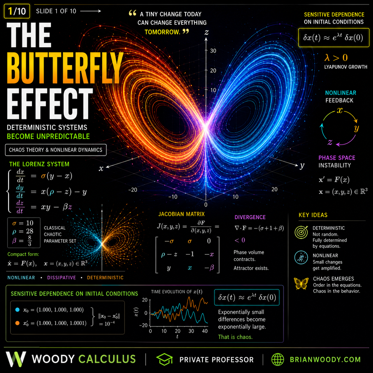
01 / 10 · The butterfly effect
A simple rule can amplify small uncertainty.
Read the explanation
02 / 10 · The Lorenz system
Three coupled nonlinear equations describe the model.
Read the explanation
03 / 10 · Sensitive dependence
Exponential separation is an average small-error model; finite gaps eventually saturate.
Read the explanation
04 / 10 · The geometry of the attractor
A typical chaotic orbit is aperiodic; projected curves can cross.
Read the explanation
05 / 10 · Lyapunov exponents
Use infinitesimal tangent perturbations to measure long-run growth.
Read the explanation
06 / 10 · The butterfly effect in action
Sensitivity is model-dependent; nonlinearity alone does not establish chaos.
Read the explanation
07 / 10 · The predictability horizon
The approximately 40-unit estimate assumes a particular starting error and tolerance. Useful statistics may remain predictable.
Read the explanation
08 / 10 · Strange attractors
The value near 2.06 is a numerical dimension estimate, not a proof.
Read the explanation
09 / 10 · Structure inside chaos
The visual box-counting table illustrates scaling; it is not a validated dimension computation.
Read the explanation
10 / 10 · Keep learning with Woody
Connect the visual patterns to methods, worked examples, and deliberate practice.
Read the explanationThese original slides introduce the ideas. Their captions and the written lesson clarify the assumptions behind forecast horizons, finite-error growth, and numerical dimension estimates.
What is the butterfly effect?
The butterfly effect is sensitive dependence on initial conditions: in a chaotic system, almost identical starting states can develop substantially different future trajectories. The equations remain deterministic; the practical limitation is uncertainty in the starting information.
While the separation is small, a useful average model is
Here represents an average exponential stretching rate. A finite pair separates unevenly and eventually saturates in a bounded region, so this approximation does not apply indefinitely.
Keep the distinction: chaos describes deterministic evolution with sensitive behavior. A stochastic model explicitly includes random variables or noise. Both kinds of models can have mathematical structure.
Edward Lorenz and the discovery of chaos
In the early 1960s, meteorologist Edward Lorenz found that restarting a weather simulation with rounded starting data could produce a very different later trajectory. The model’s equations had not changed; the initial information had.
The story illustrates a central lesson of nonlinear dynamics: excellent short-term agreement does not guarantee an accurate long-term trajectory. The famous three-equation Lorenz system provides a compact model for studying this behavior. It is a simplified convection model, not a complete operational weather forecast.
The Lorenz system: three equations, coupled motion
The classical Lorenz system is
The video uses the familiar parameters
The products and couple the coordinates nonlinearly. For these parameters, a typical chaotic trajectory remains bounded and aperiodic. Exceptional equilibrium and periodic trajectories also exist. Nonlinearity alone does not imply chaos.
The video illustrates motion starting at . Substituting into the vector field gives the initial direction:
This connects Differential Equations with Linear Algebra: the nonlinear equations drive the motion, while Jacobians and local linearization describe the evolution of small perturbations.
Sensitive dependence: two nearby starting states
The original written example compares
Each coordinate differs by , so the initial Euclidean separation is . The two solutions initially look close. Their separation can then grow unevenly, with an average exponential trend while the difference remains small.
A commonly quoted numerical estimate for the classical Lorenz system is per model time unit. The video’s longer numerical experiment gives approximately , reported aloud as . These are numerical estimates, not exact constants.
Video and written examples complement each other. The video uses the illustrative start and a separate five-pair precision experiment. The starting pair above is the written lesson’s example. In the video’s error ladder, the plotted curves show the -coordinates, but the crossing criterion uses the full three-dimensional gap.
The geometry of the Lorenz attractor
The familiar butterfly shape lives in three-dimensional phase space: a point represents the full state . A typical chaotic orbit moves around the two wings without settling into a repeating cycle, while remaining in a bounded region.
An aperiodic solution cannot return to precisely the same full three-dimensional state: uniqueness would make the subsequent motion repeat. Curves can nevertheless cross in a two-dimensional projection. A crossing on your screen is not necessarily an intersection in phase space.
Chaos can retain geometry. Detailed futures separate, yet the recognizable attractor structure remains.
Lyapunov exponents: measuring the stretching rate
Along a solution , an infinitesimal tangent perturbation satisfies the variational equation
For a generic initial direction, the largest Lyapunov exponent is
when the limit exists. Numerically, periodically rescale the tangent vector and add the logarithms of its growth factors. Divide the accumulated logarithmic growth by elapsed time. Rescaling is bookkeeping for the perturbation; it does not reset the underlying orbit.
The supplied video notes report the measured spectrum
The notes describe a fourth-order Runge–Kutta calculation with a 0.001 time step, a 100-unit warm-up, tangent QR every 0.1 unit, and 20,000 measured units. A comparison run at step 0.002 gave a slightly different largest exponent. Treat the displayed values as numerical estimates with finite-time and numerical error.
A positive exponent is not, by itself, a proof of chaos. For example, expands perturbations but does not describe bounded chaotic motion. Interpret the exponent alongside the system’s dynamics and geometry.
How can volume shrink while distances grow?
Differentiate each component in its own coordinate:
A material volume transported by the flow therefore obeys
At half a model time unit, , so about 0.1077% of the original material volume remains. Stretching in one direction can coexist with stronger contraction in others.
The sum of the Lyapunov exponents equals the time-averaged divergence; here
The rounded estimates provide a useful consistency check. Their negative sum describes net volume contraction; this check alone does not prove chaos. The animated cloud samples a material volume. Its convex hull is not that material volume, and a positive volume has not literally become a surface at finite time.
The butterfly effect in action
The butterfly-and-tornado image is a metaphor for sensitivity, not a calculation assigning one storm to one wingbeat. In a chaotic model, small uncertainty can grow substantially even though the equations remain fixed.
Chaos theory informs weather and climate modeling, fluid dynamics, engineering, biological rhythms, and orbital motion. Researchers also study nonlinear dynamics in economics and neuroscience. Whether a particular real system is chaotic requires evidence and an appropriate model; a complicated graph or nonlinear equation alone is not enough.
Derive the predictability horizon
Choose an initial uncertainty , a tolerance , and a positive average growth rate . The estimated horizon is the time when the small-error model reaches that tolerance.
- Set the error equal to the tolerance. .
- Divide by the starting error. .
- Take natural logarithms. .
- Solve for time.
What does a better measurement buy?
If the starting error is reduced by a factor , subtract the old horizon from the new one:
With the video’s estimate , a tenfold improvement adds about 2.54 model units; a hundredfold improvement adds about 5.08; a millionfold improvement adds about 15.25. These are dimensionless model time units, not weather days.
| Initial error | Average horizon | Computed first crossing |
|---|---|---|
| 10⁻² | 5.08 | 5.15 |
| 10⁻⁴ | 10.17 | 9.00 |
| 10⁻⁶ | 15.25 | 13.62 |
| 10⁻⁸ | 20.34 | 20.27 |
| 10⁻¹⁰ | 25.42 | 24.21 |
Computed crossings are the numerical results reported in the supplied lesson notes. They use the full spatial gap reaching 1. Actual finite-pair behavior fluctuates around the average model; these times are not universal constants.
The original machine-precision example
As an illustrative normalized calculation, take tolerance 1, starting error , and :
Machine epsilon describes floating-point spacing near one. It is not automatically the initial physical measurement error. The approximately 39.8-unit estimate depends on the chosen normalization and tolerance.
A horizon is a tolerance crossing, not the end of all useful prediction. Near this estimated time, detailed trajectory uncertainty reaches the chosen threshold. Statistical or geometric predictions may remain useful.
Try the formula
How much more forecast time?
Change one quantity and see what happens to the average exponential estimate. Use the same units for initial error and tolerance.
Estimated horizon: model time units
Extra time from better measurement: model time units
This calculator uses a constant average rate. It does not integrate the Lorenz equations or predict an exact first-crossing time.
Strange attractors, Poincaré sections, and dimension
A strange attractor combines attracting behavior with intricate geometry. For the classical Lorenz dynamics, typical trajectories are aperiodic, even though exceptional periodic trajectories can occur within the dynamical structure.
The video records intersections with the plane , keeping only upward crossings. This Poincaré section helps reveal the structure that can be hard to see in the full three-dimensional flow.
For the measured Lyapunov spectrum, the Kaplan–Yorke estimate is
The value near 2.06 suggests geometric complexity beyond a smooth surface without filling a solid volume. This numerical estimate is not a proof of a Hausdorff or box-counting dimension, and it should not automatically be assigned to the Poincaré section itself.
Set · Divide · Log · Solve
Three worked examples to make the method reproducible
These practice problems expand the supplied lesson notes. They are additional written exercises; the video does not individually work through all three.
1. Estimate a forecast horizon
Use , , and tolerance .
Show the complete setup and solution
Pattern: a growing exponential reaches a chosen threshold. Method: isolate the exponential and use a natural logarithm.
Check: . The estimated horizon is about 10.65 model time units.
2. Improve the starting measurement a thousandfold
Keep and the same tolerance. Reduce the starting error by a factor of 1000.
Show why the gain is additive
The new error is . Subtract the old horizon from the new one:
Check: in the average model. A thousandfold accuracy improvement adds about 8.63 model units; it does not multiply the original horizon by 1000.
3. Find when material volume reaches 1%
For the classical Lorenz parameters, use .
Show the decay calculation
Check: . This is a material-volume calculation; it does not say every distance has fallen to 1%.
Your chaos theory formula guide
- Average small-error growth
- , while the gap remains small.
- Forecast horizon
- , for and .
- Extra time from a factor-q improvement
- , with .
- Classical Lorenz volume contraction
- .
- Kaplan–Yorke estimate for this spectrum
- .
Common mistakes to catch
- Using the exponential separation model after a finite gap has saturated.
- Treating an eigenvalue at one equilibrium as a long-run Lyapunov exponent.
- Assuming negative divergence contracts every distance.
- Calling a numerical dimension estimate a proof.
- Reading dimensionless Lorenz time units as weather days.
- Confusing a projected crossing with a repeated full state.
Continue with how differential equations give rise to chaos, phase portraits and stability, and fractals and dimension.
Where this connects to your course
- Differential Equations: nonlinear systems, phase portraits, equilibrium points, stability, and long-term behavior.
- Calculus 3: partial derivatives, vector fields, divergence, and three-dimensional geometry.
- Linear Algebra: Jacobians, tangent dynamics, stretching, and contractions.
- Calculus 2: exponential models, logarithms, approximation, convergence, and integration.
- Real Analysis: limits, continuity, convergence, and precise statements about numerical evidence.
- Abstract Algebra: a related habit of studying structure and transformations; group theory is not a prerequisite for this lesson.
- Calculus 1 foundations: derivatives, rates of change, and tangent behavior used in the models above.
Practice the Woody method
Pattern first. Setup second. Computation third. First recognize an exponential threshold problem. Then choose logarithms, write the full setup, and solve.
- Write the Lorenz equations and identify the two nonlinear product terms.
- Explain how deterministic motion can still be sensitive to uncertain starting data.
- Reproduce the forecast-horizon derivation without looking.
- Work the three examples above and check each by substitution.
- Rewrite a correct solution 3–5 times while saying each step confidently aloud.
- Explain why shrinking volume and growing distances can happen together.
Perfect practice makes perfect. Check the solution first, then practice the correct reasoning. Return to it later and see whether you can rebuild the setup on your own.
Questions students ask about chaos theory
What is chaos theory?
Chaos theory studies deterministic dynamics with sensitive dependence and complex long-term behavior. Knowing the equations does not eliminate uncertainty in the starting state or guarantee accurate detailed forecasts indefinitely.
What does the butterfly effect mean in mathematics?
It means sensitive dependence on initial conditions. Small initial differences can grow substantially. Exponential growth is an average small-error model, not an exact law that continues forever for a finite pair.
What is the Lorenz system?
It is a three-variable nonlinear differential equation model derived from simplified convection. At the classical parameters 10, 28, and 8/3, it supports chaotic dynamics. A typical chaotic trajectory is bounded and aperiodic, while exceptional equilibrium and periodic trajectories also exist.
What do Lyapunov exponents measure?
They measure long-run average exponential growth rates of infinitesimal tangent perturbations. Numerical algorithms repeatedly rescale perturbations and accumulate logarithmic growth. A positive exponent is evidence of stretching, but alone does not prove chaos.
Does better measurement make prediction possible forever?
No. In the average exponential model, reducing the starting error by a factor q adds approximately ln(q)/lambda to the forecast horizon. The result also depends on the error tolerance and the model being used.
Can nearby solutions separate while volume shrinks?
Yes. A region can stretch in one direction while contracting more strongly in others. The classical Lorenz divergence is -41/3, so transported material volume contracts even while typical nearby trajectories separate.
Is chaos the same as randomness?
No. Chaotic models evolve deterministically from an exact state. Stochastic models explicitly include random variables or noise. Both kinds of models can have mathematical structure.
Is the butterfly effect real or just a metaphor?
Sensitive dependence is a mathematical property of many dynamical models. The butterfly-and-tornado image is a metaphor. Applying the idea to a particular physical system requires an appropriate model and evidence.
What is a strange attractor?
It is an attracting structure with intricate, often fractal geometry. In the Lorenz example, typical chaotic motion is aperiodic. That does not mean the attractor contains no exceptional periodic trajectories.
Is the Lorenz attractor dimension exactly 2.06?
No. The value near 2.06 used here is a numerical Kaplan-Yorke estimate derived from the Lyapunov spectrum. It is not an exact constant or a proof of Hausdorff or box-counting dimension.
How is this connected to Differential Equations?
The Lorenz equations define the flow. Derivatives and the Jacobian describe tangent dynamics, while exponents, divergence, and phase-space geometry help describe its behavior.
Do the video and written lesson use the same examples?
They use complementary examples. The video illustrates the state (2, -1, 16) and a five-pair error ladder. The article retains its original starting-pair and machine-precision examples and adds three practice problems with worked solutions.
Your next step with Woody
Make the setup feel as familiar as the answer
If you can follow the animation but still freeze when it is your turn to choose a method, that is where practice and teaching support matter. In Woody Calculus & Advanced Mathematics Mastery Lab, keep building your mathematics with my lessons and personal teaching expertise.
I’m Brian M. Woody, a former university instructor with more than 25 years of teaching experience. We work from the pattern to the method, then build a setup you can explain and reproduce.
Start your FREE 7-day trialExplore the program before deciding whether it fits your course and the way you want to learn.
Learn the patterns. Learn the game. Solve with confidence.