Fractals Explained
How simple rules create infinite mathematical structure.
Fractals are not merely psychedelic pictures or objects that “look complicated.”
They are mathematical structures organized across scales. Some are built by exact
self-similarity, some emerge from repeated iteration, some have non-integer
dimension, and some form the boundaries of chaotic dynamical systems. This lesson
develops the mathematics from the ground up: definition, iteration, the Mandelbrot
set, escape orbits, Julia sets, fractal dimension, chaos, natural patterns, myths,
worked examples, and mastery tasks.
Reading level: layered for curious beginners, high-school and
undergraduate students, and advanced readers who want the precise mathematics.
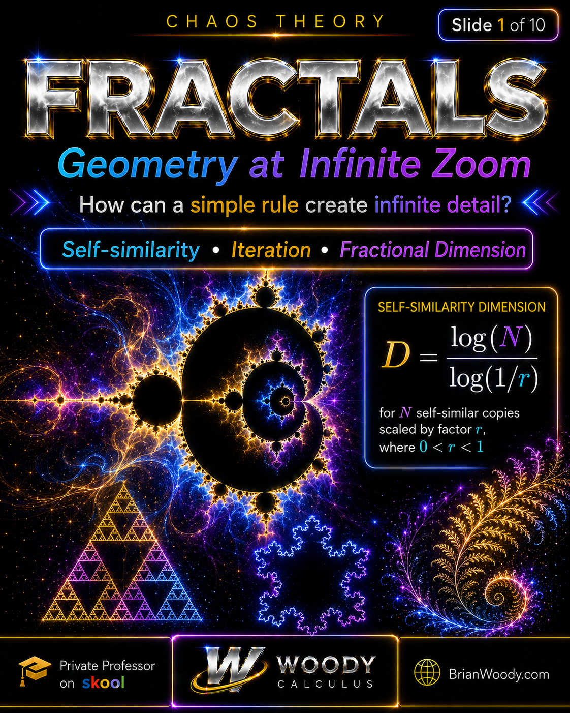
dimension, the Mandelbrot set, and geometric structure revealed at
progressively smaller scales.
What Is a Fractal?
A fractal is a mathematical set or geometric object with
meaningful structure across scales. Magnifying it continues to reveal
organized detail. Classical fractals often display exact self-similarity and
may have a non-integer dimension, while other fractals—such as the Mandelbrot
set—have more complicated, nonrepeating local structure.
There is no single elementary checklist that captures every object called a
fractal. Exact self-similarity is common but not universal. Non-integer dimension
is common but not required. The most reliable unifying idea is that ordinary
Euclidean geometry does not adequately describe how the object’s detail behaves
as scale changes.
Complexity does not require a complicated rule. Repetition,
scaling, and feedback can turn a short instruction into geometry with
inexhaustible mathematical depth.
What Makes a Fractal a Fractal?
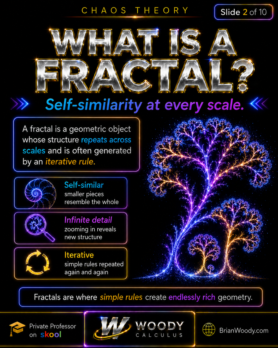
showing exact, approximate, or statistical self-similarity and detail
revealed by magnification.
The word fractal is used for several related kinds of mathematical
objects. The following properties are common, but no single one is a complete
universal definition.
-
Structure across scales: magnification reveals additional
organized detail rather than a featureless smooth object.
-
Self-similarity: smaller portions may resemble the whole.
The resemblance can be exact, approximate, or statistical.
-
Iterative construction: many fractals arise by applying
the same transformation repeatedly.
-
Unusual dimension: a fractal may occupy space in a way that
is more substantial than a line but less complete than a surface.
-
Fine boundary structure: some fractals appear as boundaries
separating different dynamical behaviors.
Exact, Approximate, and Statistical Self-Similarity
| Type | Meaning | Example |
|---|---|---|
| Exact self-similarity | Scaled pieces reproduce the whole exactly. | Cantor set, Koch curve, Sierpiński triangle |
| Approximate self-similarity | Smaller pieces resemble the whole but are not exact copies. | Many branching biological structures |
| Statistical self-similarity | Scaling laws persist statistically rather than point by point. | Idealized models of coastlines, clouds, and rough surfaces |
| Complex multiscale structure | New local structure appears at each scale without exact global repetition. | Mandelbrot set |
The Mandelbrot set is often casually called self-similar, but it is not
globally exactly self-similar like the Cantor set. Its boundary contains
repeated and near-repeated structures, including miniature Mandelbrot-like
copies, while different locations reveal genuinely different geometry.
A Short History of Fractal Geometry
Fractal geometry did not appear in one moment. It grew from several mathematical
objects that challenged the smooth geometry of points, lines, curves, and
surfaces.
Georg Cantor: the middle-thirds Cantor set showed that an
uncountable set can have total length zero and can reproduce itself at
smaller scales.
Helge von Koch: the Koch curve supplied an elementary
geometric example of a continuous curve with no tangent, infinite length,
and exact self-similarity.
Wacław Sierpiński: recursive constructions such as the
Sierpiński triangle revealed systematic holes and non-integer scaling
behavior.
Gaston Julia and Pierre Fatou: early twentieth-century
work on iterated complex functions established the foundations of what is
now called complex dynamics.
Benoît Mandelbrot: in the 1970s and early 1980s,
Mandelbrot helped unite these previously isolated examples under the
language of fractal geometry and used emerging computer graphics to reveal
the extraordinary structures produced by iteration.
See the
MacTutor History of Fractal Geometry
for a documented historical overview.
Iteration: The Engine Behind Fractals
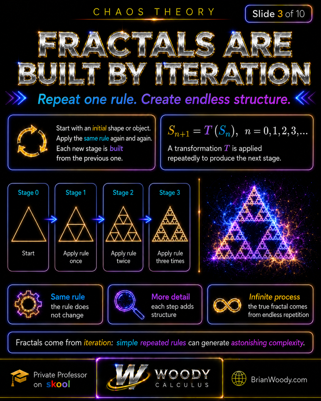
producing an orbit or sequence of stages in which simple rules can
generate increasingly complex fractal structure.
An iteration feeds the output of one step back into the same
rule. If the transformation is denoted by \(T\), then a sequence of stages
can be written as
S_{n+1}=T(S_n),
\qquad n=0,1,2,\ldots
\]
In dynamical systems, the resulting sequence
x_0\longmapsto x_1\longmapsto x_2\longmapsto x_3\longmapsto\cdots
\]
is called the orbit of the initial point. An orbit may settle
to a fixed point, enter a periodic cycle, remain bounded without repeating, or
escape without bound.
Iteration Is Not the Same as Recursion
The words are closely related but emphasize different viewpoints. A recursive
definition describes an object in terms of earlier stages. Iteration emphasizes
repeatedly applying a transformation. Many fractal constructions can be
described both ways.
Example: The Sierpiński Triangle
Begin with a filled equilateral triangle.
Divide it into four congruent triangles.
Remove the central triangle.
Repeat the same operation on every remaining triangle.
After each step, three copies remain, each scaled by a factor of one half. That
scaling information will later determine the Sierpiński triangle’s dimension.
What Is the Mandelbrot Set?
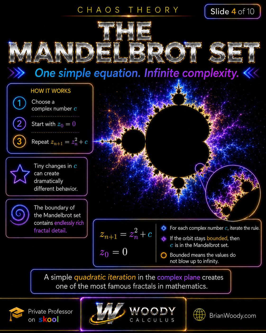
which the orbit of zero under z sub n plus one equals z sub n squared
plus c remains bounded.
For each complex number \(c\), define the quadratic function
f_c(z)=z^2+c.
\]
Start at the critical point \(z_0=0\), then iterate:
z_0=0,
\qquad
z_{n+1}=z_n^2+c.
\]
The parameter \(c\) belongs to the Mandelbrot set when the orbit
\((z_n)\) remains bounded.
\boxed{
M=
\left\{
c\in\mathbb C:
\bigl(f_c^n(0)\bigr)_{n\ge0}
\text{ remains bounded}
\right\}
}.
\]
The Mandelbrot set is not one orbit. It is a map of an entire
parameter plane. Every point \(c\) defines a different
quadratic dynamical system, and the picture records which of those systems
keep the critical orbit bounded.
How a Computer Draws the Mandelbrot Set
A computer assigns one complex parameter \(c=a+bi\) to each pixel, runs the
iteration, and checks whether the orbit escapes. Outside points are often
colored according to how quickly they escape. Points that have not escaped
after a chosen iteration limit are drawn as if they belong to the set,
producing a numerical approximation.
for each pixel:
    convert pixel position to c = a + bi
    z = 0

    repeat up to MAX_ITERATIONS:
        z = z*z + c

        if abs(z) > 2:
            color by escape time
            stop

    if no escape was detected:
        color as an unresolved bounded point
Failing to escape after finitely many steps does not by itself prove that a
point belongs to the Mandelbrot set. A rendered image is a finite numerical
approximation to an infinite mathematical definition.
How the Mandelbrot Escape Test Works
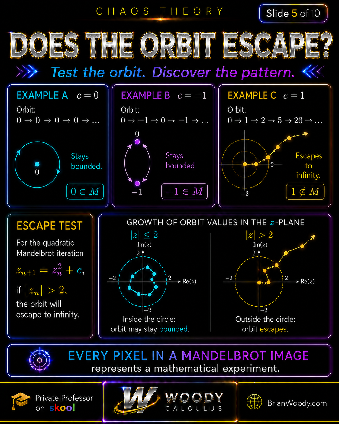
orbits, while c equals one escapes; once an orbit value has modulus
greater than two, the quadratic Mandelbrot orbit diverges.
Example A: \(c=0\)
0\longmapsto0\longmapsto0\longmapsto\cdots
\]
The orbit is bounded, so
0\in M.
\]
Example B: \(c=-1\)
0\longmapsto-1\longmapsto0\longmapsto-1\longmapsto\cdots
\]
The orbit enters a period-two cycle, so
-1\in M.
\]
Example C: \(c=1\)
0\longmapsto1\longmapsto2\longmapsto5\longmapsto26\longmapsto\cdots
\]
The orbit escapes to infinity, so
1\notin M.
\]
Why the Escape Radius Is 2
First suppose \(|c|\le2\). If an iterate satisfies \(|z_n|>2\), then the
reverse triangle inequality gives
|z_{n+1}|
=|z_n^2+c|
\ge |z_n|^2-|c|
\ge |z_n|^2-2.
\]
Subtracting 2 from both sides yields
|z_{n+1}|-2
\ge |z_n|^2-4
=\bigl(|z_n|-2\bigr)\bigl(|z_n|+2\bigr)
>4\bigl(|z_n|-2\bigr).
\]
Therefore, for every integer \(k\ge1\),
|z_{n+k}|-2
>4^k\bigl(|z_n|-2\bigr).
\]
The right-hand side tends to infinity, so \(|z_{n+k}|\to\infty\). This
proves escape when \(|c|\le2\).
Now suppose \(|c|>2\). Since \(z_1=c\),
|z_2|
=|c^2+c|
=|c|\,|c+1|
\ge |c|\bigl(|c|-1\bigr)
>|c|.
\]
Whenever \(|z_n|\ge|c|>2\),
|z_{n+1}|
\ge |z_n|^2-|c|
\ge |z_n|^2-|z_n|
=|z_n|\bigl(|z_n|-1\bigr)
\ge \bigl(|c|-1\bigr)|z_n|.
\]
Because \(|c|-1>1\), the magnitudes grow at least geometrically. Hence this
case also escapes to infinity.
\boxed{
|z_n|>2
\quad\Longrightarrow\quad
|z_m|\to\infty\text{ as }m\to\infty
}
\]
Choose a complex parameter \(c\).
Set \(z_0=0\).
Repeat \(z_{n+1}=z_n^2+c\).
If an iterate satisfies \(|z_n|>2\), stop: the orbit will escape
and \(c\notin M\).
If no escape is detected after the chosen iteration limit, mark the
pixel as unresolved or provisionally bounded. More iterations improve
the approximation near the boundary.
Mandelbrot Set vs. Filled Julia Set vs. Julia Set
The Mandelbrot set and Julia sets are built from the same quadratic family,
but they answer different questions.
The Mandelbrot Set Varies the Parameter
In the Mandelbrot set, we vary the parameter \(c\), always begin with the
critical point \(z_0=0\), and ask whether that one critical orbit remains
bounded.
M=
\left\{
c\in\mathbb C:
\bigl(f_c^n(0)\bigr)_{n\ge0}
\text{ is bounded}
\right\}.
\]
The Filled Julia Set Fixes \(c\) and Varies the Initial Point
Fix one parameter \(c\). The filled Julia set \(K_c\)
consists of all initial points whose orbits remain bounded:
\boxed{
K_c=
\left\{
z_0\in\mathbb C:
\bigl(f_c^n(z_0)\bigr)_{n\ge0}
\text{ remains bounded}
\right\}
}.
\]
The Julia Set Is the Boundary
The Julia set is not the entire bounded-orbit region. It is
the boundary of the filled Julia set:
\boxed{J_c=\partial K_c}.
\]
This boundary separates qualitatively different orbit behavior and is where
the most intricate complex dynamics occur.
| Object | What Varies? | Question | Plane |
|---|---|---|---|
| Mandelbrot set \(M\) | Parameter \(c\) | Does the critical orbit of zero remain bounded? | Parameter plane |
| Filled Julia set \(K_c\) | Initial point \(z_0\), with \(c\) fixed | Which initial orbits remain bounded? | Dynamical plane |
| Julia set \(J_c\) | Boundary points, with \(c\) fixed | Where is the boundary between dynamical behaviors? | Dynamical plane |
For the quadratic family \(f_c(z)=z^2+c\), the Julia set is connected
exactly when the critical parameter belongs to the Mandelbrot set:
\boxed{
c\in M
\quad\Longleftrightarrow\quad
J_c\text{ is connected}
}.
\]
See
Julia Sets and the Mandelbrot Set
for a concise mathematical introduction to bounded orbits, filled Julia
sets, Julia sets, connectedness, and the Mandelbrot criterion.
What Is Fractal Dimension?
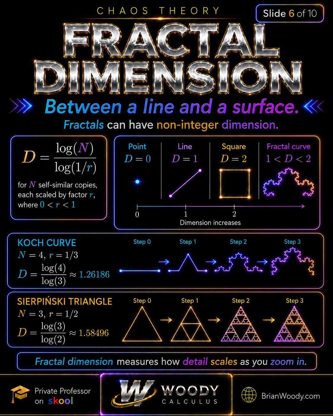
dimensions; the Koch curve has dimension log four over log three, and
the Sierpinski triangle has dimension log three over log two.
Ordinary Euclidean dimension counts independent directions:
\text{point: }D=0,
\qquad
\text{line: }D=1,
\qquad
\text{plane: }D=2,
\qquad
\text{space: }D=3.
\]
Fractal dimension asks a different scaling question: how rapidly does the
amount of visible structure grow as the measuring scale becomes smaller?
The Similarity-Dimension Formula
Suppose an exactly self-similar object consists of \(N\) congruent copies,
The Koch curve contains four self-similar copies, each scaled by one third:
The curve is more space-filling than an ordinary line but does not fill a
The Sierpiński triangle contains three copies, each scaled by one half:
The formula \(D=\log N/\log(1/r)\) applies directly to equal-scale
A fractal is a geometric object or set.
The rule is deterministic, but orbit behavior can change dramatically as the The Lorenz equations are
For classical parameter choices, trajectories can approach the Lorenz strange
Chaos describes how a system evolves; fractals can describe the
Why should the dimension formula be \(D=\log N/\log(1/r)\)? The
If an object has dimension \(D\) and is scaled by a linear factor \(r\), Now solve for \(D\):
Divide a square into four smaller squares, each scaled by one half. Then
The scaling formula correctly reproduces the ordinary dimension of a square.
The middle-thirds Cantor set contains two self-similar copies, each scaled by
It is more substantial than a finite or countable collection of isolated
The Koch curve is a curve, but its detail grows too quickly to behave like a
For the full real-analysis story—uncountability, zero length, perfectness,
Similarity dimension is elegant but specialized. Box-counting and Hausdorff
Cover a set \(E\) with a grid of boxes of side length \(\varepsilon\).
If the ordinary limit fails to exist, mathematicians use upper and lower
Hausdorff dimension permits coverings by sets of varying sizes rather than
The Hausdorff dimension is the critical value of \(s\) where the associated
The Mandelbrot set contains interior, so the set itself has Hausdorff
A set can therefore have the full Hausdorff dimension of the plane while
See Mitsuhiro Shishikura,
Begin with an equilateral triangle of side length one. At every stage of the The stage-\(n\) perimeter is Since \(4/3>1\),
Let \(A_0=\sqrt3/4\) be the area of the original triangle. The total
The Koch snowflake encloses a finite area even though its boundary has
Nature often displays branching, roughness, and scale-dependent patterns
Measuring a coastline with a shorter ruler typically produces a larger
Benoît Mandelbrot,
Mathematical fractals can continue forever. Physical nature
Fractal methods are useful when shape, roughness, branching, or complexity
Fractals matter because they connect ideas that appear separate in an
Fractals show us that complexity can be born from
Close the article before doing these. Retrieval is part of learning.
Rewrite perfect solutions. Speak every transition. If you cannot explain why
A fractal is a mathematical set or shape with organized structure across
Common characteristics include structure across scales, exact or
The Mandelbrot set is the set of complex parameters c for which the orbit
Start with z zero equal to zero and repeatedly calculate z sub n plus one
Once an orbit value has modulus greater than two, the excess above radius
Not automatically. In a finite rendering, black often means only that the
The Mandelbrot set varies the parameter c and tests the critical orbit
The filled Julia set K sub c contains all initial points with bounded
Fractal dimension measures how an object’s detail or space-filling behavior
Dimension can be defined through scaling rather than only by counting
The middle-thirds Cantor set has similarity and Hausdorff dimension log 2
The Koch curve has dimension log 4 over log 3, approximately 1.26186, so
Yes. Non-integer dimension is common but not required. A deep theorem
No. Fractals describe geometric structure, while chaos describes
Many natural structures show approximate or statistical fractal behavior
As a mathematical set, its boundary has structure at arbitrarily small
No single person invented every fractal idea. Cantor, von Koch,
Fractal methods are used in procedural graphics, scaling analysis,
each scaled by a factor \(r\), where \(0
\boxed{
D=\frac{\log N}{\log(1/r)}
}.
\]
Koch Curve
N=4,
\qquad
r=\frac13,
\qquad
D=\frac{\log4}{\log3}\approx1.26186.
\]
plane:
1Sierpiński Triangle
N=3,
\qquad
r=\frac12,
\qquad
D=\frac{\log3}{\log2}\approx1.58496.
\]
self-similar objects under suitable separation conditions. More general
fractals require broader notions such as box-counting or Hausdorff
dimension.
How Fractals Connect to Chaos Theory
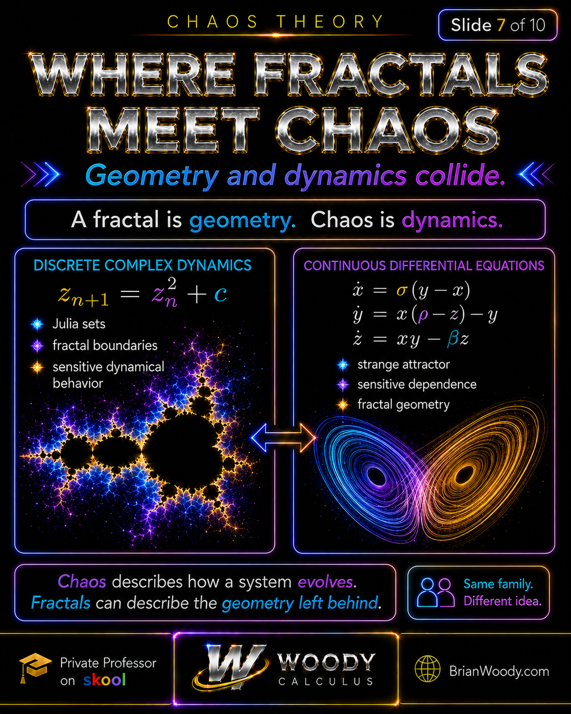
dynamics; complex iteration and nonlinear differential equations can
produce fractal boundaries and strange attractors.
Chaos describes long-term dynamical behavior, especially
deterministic systems with sensitive dependence on initial conditions.
The subjects overlap because chaotic systems often produce fractal
invariant sets, basin boundaries, and strange attractors.
Discrete Complex Dynamics
z_{n+1}=z_n^2+c.
\]
parameter or initial point changes. Julia sets form fractal boundaries between
different dynamical regions.
Continuous Dynamics: The Lorenz System
\dot x=\sigma(y-x)
\]
\dot y=x(\rho-z)-y
\]
\dot z=xy-\beta z.
\]
attractor. The evolution is deterministic, yet nearby initial states separate
rapidly, and the attractor has fractal geometric structure.
geometry organized by that evolution.
Continue the Chaos Theory Cluster
Deriving Fractal Dimension From Self-Similarity
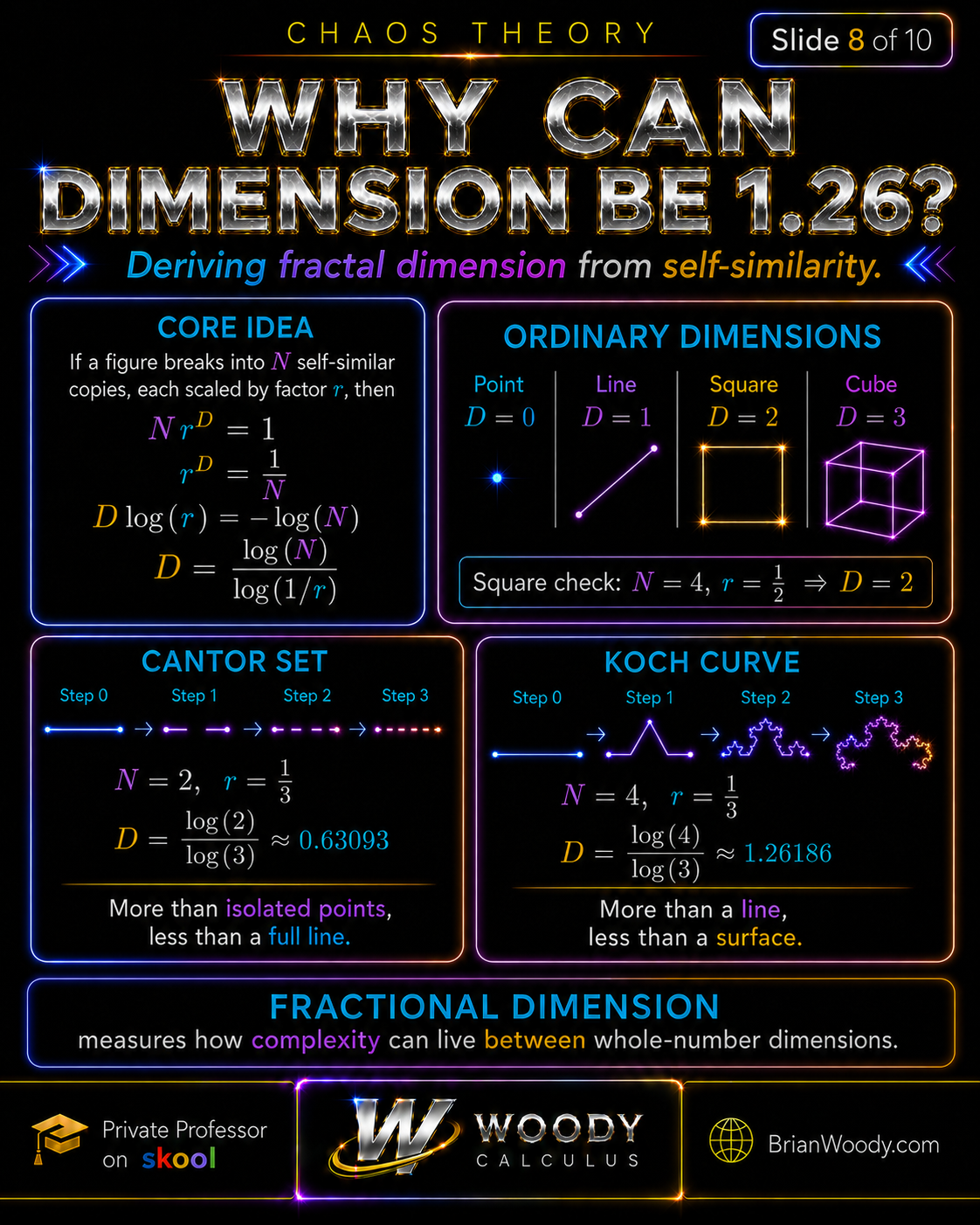
becomes log N divided by log of one over r; the Cantor set has dimension
about 0.63093 and the Koch curve about 1.26186.
derivation comes from the scaling law for ordinary dimension.
Start With Ordinary Scaling
then its \(D\)-dimensional size scales by \(r^D\). If \(N\) scaled copies
exactly rebuild the original object, their total scaled size must equal one
original object:
Nr^D=1.
\]
r^D=\frac1N.
\]
D\log r=-\log N.
\]
\boxed{
D=\frac{\log N}{\log(1/r)}
}.
\]
Trust Check: Does the Formula Recover a Square?
N=4,
\qquad
r=\frac12,
\qquad
D=\frac{\log4}{\log2}=2.
\]
Cantor Set: Dimension Below 1
one third:
\boxed{
D_{\text{Cantor}}
=\frac{\log2}{\log3}
\approx0.63093
}.
\]
points, yet it occupies less of the line than a full one-dimensional
interval.
Koch Curve: Dimension Above 1
\boxed{
D_{\text{Koch}}
=\frac{\log4}{\log3}
\approx1.26186
}.
\]
smooth one-dimensional object.
nowhere density, and self-similarity—read
The Cantor Set: Infinite Points, Zero Length, and Real Analysis
.
Box-Counting Dimension and Hausdorff Dimension
dimension apply to much broader classes of sets.
Box-Counting Dimension
Let \(N(\varepsilon)\) be the number of boxes needed to intersect the set.
If the limit exists, the box-counting dimension is
\boxed{
\dim_B(E)
=
\lim_{\varepsilon\to0}
\frac{\log N(\varepsilon)}{\log(1/\varepsilon)}
}.
\]
box-counting dimensions defined with limsup and liminf.
Hausdorff Dimension
one fixed grid. For each exponent \(s\), it studies sums of the form
\sum_i\bigl(\operatorname{diam}U_i\bigr)^s.
\]
Hausdorff measure changes from infinity to zero. This definition is
technically deeper, but it is powerful enough to distinguish very irregular
sets.
A Deep Mandelbrot Fact
dimension two. More surprisingly, Shishikura proved that its boundary also
has Hausdorff dimension two:
\boxed{
\dim_H(\partial M)=2
}.
\]
still being a boundary with extraordinarily intricate local structure.
The Hausdorff Dimension of the Boundary of the Mandelbrot Set and Julia Sets
.
How Can a Fractal Have Infinite Perimeter but Finite Area?
Koch snowflake, replace each segment with four segments, each one third as
long.
Perimeter
P_n=3\left(\frac43\right)^n.
\]
P_n\to\infty.
\]
Area
added area is a convergent geometric series:
A_\infty
=
A_0\left[
1+\frac13\sum_{k=0}^{\infty}
\left(\frac49\right)^k
\right].
\]
\boxed{
A_\infty
=
\frac85A_0
=
\frac{2\sqrt3}{5}
}.
\]
infinite length. Fractal geometry separates ideas that ordinary smooth
geometry often makes us expect to move together.
Are Fractals Really Everywhere in Nature?
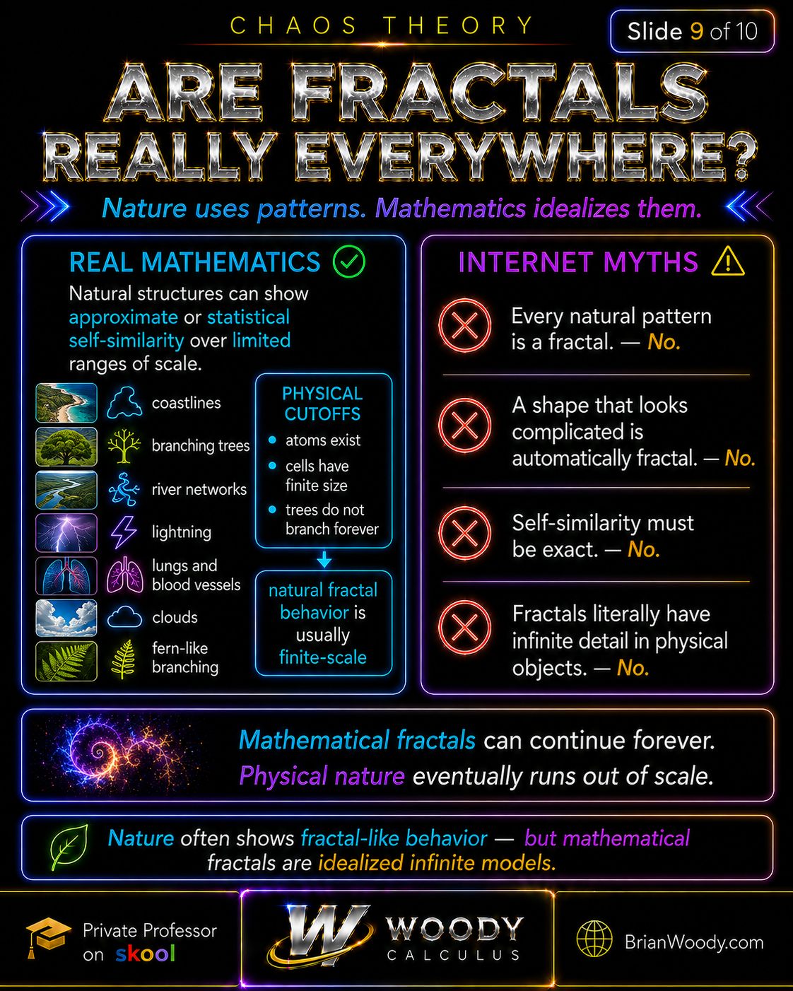
fractal behavior over limited scales, but physical objects do not
possess literally infinite detail.
that are well modeled with fractal ideas. But physical objects are not ideal
mathematical fractals extending through infinitely many scales.
Natural Structure
What the Fractal Model Captures
Physical Limitation
Coastlines
Measured length depends on the measuring scale; roughness can follow scaling laws.
Rock grains, erosion scales, maps, and measurement resolution impose cutoffs.
River networks
Branching and drainage organization across multiple scales.
Topography, geology, and finite watershed size limit the scaling range.
Trees and ferns
Repeated branching patterns and approximate self-similarity.
Cells, vascular constraints, gravity, and growth history prevent infinite repetition.
Lungs and blood vessels
Hierarchical branching used to distribute flow through space.
Biological tissues and vessel diameters have finite lower scales.
Lightning and clouds
Irregular branching or statistical roughness.
Atmospheric physics determines a finite range of observable scales.
The Coastline Paradox
measured length because the smaller ruler follows more bays, inlets, and
irregularities. Mandelbrot’s famous 1967 paper used statistical
self-similarity and fractional dimension to clarify this scale dependence.
How Long Is the Coast of Britain? Statistical Self-Similarity and Fractional Dimension
.
Myth Check
Claim
Verdict
Better Statement
Every complicated natural shape is a fractal.
False
Complex appearance alone does not establish a scaling law or fractal dimension.
Self-similarity must always be exact.
False
Natural systems often show approximate or statistical self-similarity.
Physical objects contain infinite detail.
False
Mathematical fractals can continue indefinitely; physical systems have lower and upper cutoffs.
Every spiral, branch, or rough boundary is fractal.
False
A fractal claim requires a defined scaling property, dimension, or dynamical construction.
eventually runs out of scale.
What Are Fractals Used For?
changes with scale. Applications do not require claiming that every object
is a perfect fractal.
Computer graphics and procedural generation: iterative
and recursive rules create mountains, clouds, branching vegetation,
textures, and virtual landscapes without specifying every detail by hand.
Scientific image analysis: box-counting and related
scaling measurements can quantify texture, branching, or boundary
complexity in carefully defined datasets.
Antenna engineering: self-similar geometries can produce
compact multiband designs, although the engineering performance depends
on the complete electromagnetic design rather than the word “fractal”
alone.
Geoscience and hydrology: scaling tools help analyze
rough terrain, drainage networks, shorelines, and spatial clustering over
finite ranges.
Dynamical systems: fractal basin boundaries and strange
attractors reveal how deterministic systems organize complicated
long-term behavior.
Mathematical analysis: Cantor-type sets, Hausdorff
measure, nowhere differentiable curves, and complex dynamics test and
extend the concepts of length, area, dimension, continuity, and
boundary.
Why Fractals Matter
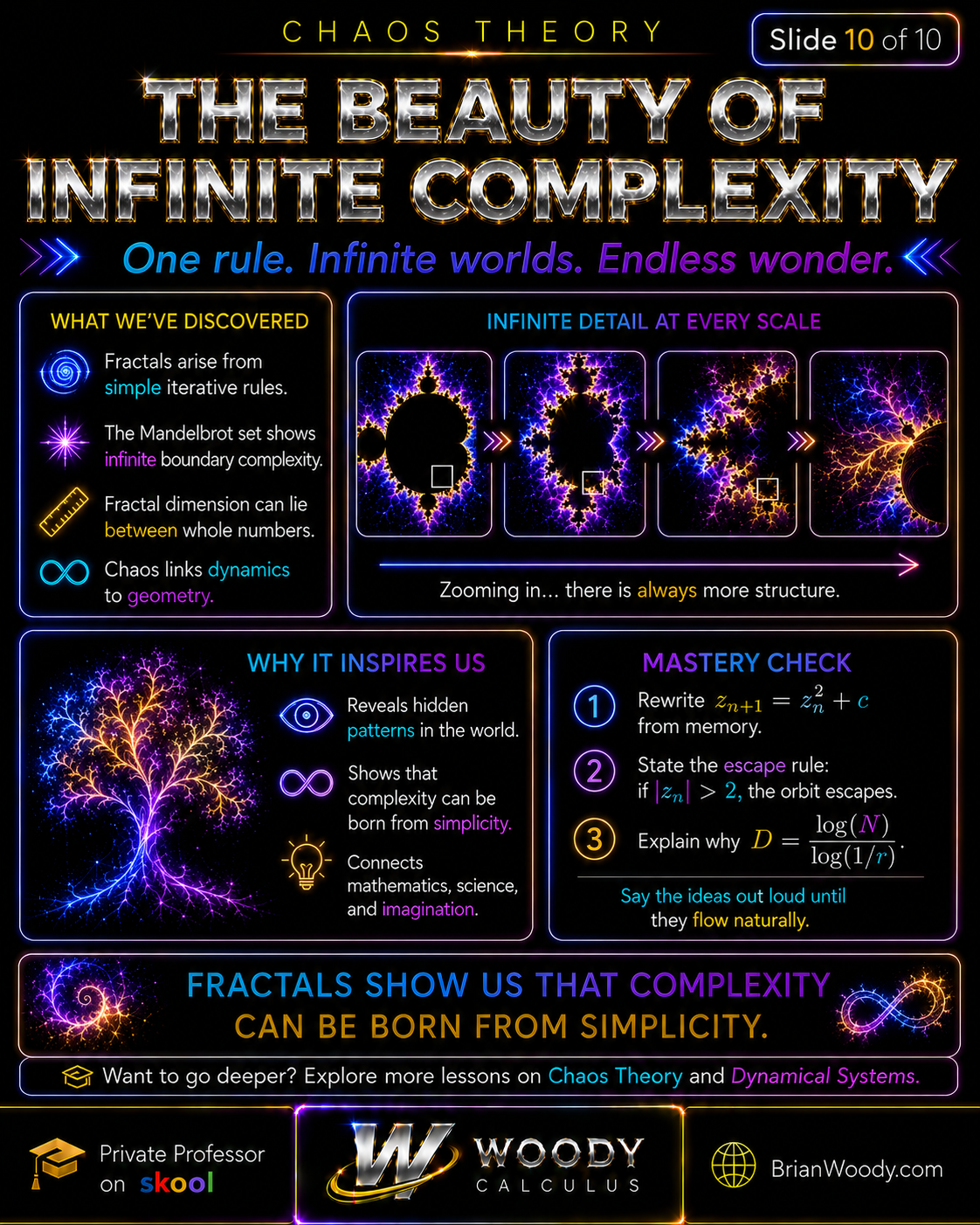
structure, fractional dimension, and connections between geometry and
dynamics; the mastery check requires active recall.
ordinary course sequence:
Geometry: scaling, self-similarity, roughness, and dimension.
Complex numbers: the dynamics of \(z^2+c\).
Sequences: orbits generated by repeated iteration.
Real analysis: limits, infinite constructions, measure, and Cantor sets.
Differential equations: strange attractors and nonlinear dynamics.
Computation: finite algorithms revealing the structure of infinite definitions.
simplicity. A short rule can generate an orbit, an orbit can
organize a boundary, and a boundary can contain structure at every
mathematically accessible scale.
Fractals Formula Sheet
General Iteration
x_{n+1}=f(x_n).
\]
Quadratic Complex Iteration
z_{n+1}=z_n^2+c.
\]
Mandelbrot Set
M=
\left\{
c\in\mathbb C:
\bigl(f_c^n(0)\bigr)_{n\ge0}
\text{ remains bounded}
\right\}.
\]
Escape Criterion
|z_n|>2
\quad\Longrightarrow\quad
\text{escape to infinity}.
\]
Filled Julia Set and Julia Set
K_c=
\left\{
z_0\in\mathbb C:
\bigl(f_c^n(z_0)\bigr)_{n\ge0}
\text{ is bounded}
\right\}.
\]
J_c=\partial K_c.
\]
Similarity Dimension
Nr^D=1.
\]
D=\frac{\log N}{\log(1/r)}.
\]
Box-Counting Dimension
\dim_B(E)
=
\lim_{\varepsilon\to0}
\frac{\log N(\varepsilon)}{\log(1/\varepsilon)}.
\]
Common Fractal Mistakes
Calling every complicated image a fractal. Complexity of
appearance is not enough; identify a scaling law, iterative construction,
dimension, or dynamical boundary.
Saying every fractal is exactly self-similar. Exact,
approximate, statistical, and more general multiscale structures must be
distinguished.
Assuming every fractal has non-integer dimension. Some
fractal sets have integer Hausdorff dimension; the boundary of the
Mandelbrot set has dimension two.
Confusing the parameter plane with the dynamical plane.
The Mandelbrot set varies \(c\); a filled Julia set fixes \(c\) and varies
\(z_0\).
Calling the filled Julia set the Julia set. The
bounded-orbit region is \(K_c\); the Julia set is the boundary
\(J_c=\partial K_c\).
Treating “did not escape after 500 iterations” as a proof of
membership. Finite escape-time rendering is a numerical
approximation.
Using the similarity-dimension formula without checking its
hypotheses. Equal-scale self-similarity and suitable separation
are needed for the direct formula.
Calling fractals and chaos synonyms. Fractals describe
geometry; chaos describes dynamical behavior. They overlap but are not the
same concept.
Claiming nature contains literal infinite detail.
Physical systems show finite-range, approximate, or statistical fractal
behavior.
Prove That You Understand Fractals
Rewrite the Mandelbrot iteration \(z_{n+1}=z_n^2+c\)
and the initial condition \(z_0=0\) from memory.
Calculate the first five orbit values for \(c=0\),
\(c=-1\), and \(c=1\), then classify each parameter.
State the escape rule aloud and explain why crossing
radius two forces the orbit to diverge.
Explain the difference among the Mandelbrot set \(M\),
filled Julia set \(K_c\), and Julia set \(J_c\) without looking back.
Derive \(D=\log N/\log(1/r)\) starting from \(Nr^D=1\).
Compute the similarity dimensions of the Cantor set,
Koch curve, and Sierpiński triangle from memory.
Say the distinction aloud until it is automatic:
chaos is dynamics; fractals are geometry.
Test a natural-fractal claim: choose one natural pattern
and state exactly what data would be needed to test finite-range fractal
scaling rather than merely asserting it.
one line becomes the next, the mathematics is not yet yours.
Fractals FAQ
What is a fractal in simple terms?
scales. Magnifying it reveals additional detail, and many classical
fractals are built from repeated scaled copies or iterative rules.
What are the main characteristics of a fractal?
approximate self-similarity, iterative construction, intricate boundaries,
and a dimension that may differ from ordinary Euclidean dimension. Not
every fractal has every one of these properties.
What is the Mandelbrot set?
of zero under the iteration z squared plus c remains bounded.
What equation generates the Mandelbrot set?
equal to z sub n squared plus c. The parameter c belongs to the Mandelbrot
set when that orbit remains bounded.
Why is the Mandelbrot escape radius equal to 2?
two grows at least geometrically, forcing the orbit’s magnitudes to diverge.
Does a black pixel prove that a point is in the Mandelbrot set?
orbit did not escape before the chosen iteration limit. Boundary points may
require much deeper computation or theoretical analysis.
What is the difference between the Mandelbrot set and a Julia set?
starting at zero. A Julia set fixes c and describes the boundary of bounded
behavior in the dynamical plane as the initial point varies.
What is the difference between a Julia set and a filled Julia set?
orbits. The Julia set J sub c is the boundary of K sub c.
What is fractal dimension?
changes with scale. Depending on the context, mathematicians use similarity,
box-counting, or Hausdorff dimension.
How can a dimension be fractional?
directions. A self-similar object made of N copies scaled by r has
similarity dimension log N divided by log of one over r, which need not be
an integer.
What is the dimension of the Cantor set?
over log 3, approximately 0.63093.
What is the dimension of the Koch curve?
its scaling behavior lies between that of a line and a surface.
Can a fractal have an integer dimension?
states that the boundary of the Mandelbrot set has Hausdorff dimension two.
Are fractals and chaos the same thing?
deterministic dynamical behavior with properties such as sensitive
dependence. Chaotic systems often produce fractal attractors or boundaries,
which is why the two subjects are closely connected.
Are fractals really found in nature?
over limited ranges of scale. Physical objects are not perfect infinite
fractals because atoms, cells, material thickness, and finite size impose
cutoffs.
Does the Mandelbrot set contain infinite detail?
scales. A computer image shows only a finite-resolution approximation of
that infinite mathematical object.
Who invented fractals?
Sierpiński, Julia, Fatou, and others created foundational examples and
theories. Benoît Mandelbrot coined the term fractal and unified the field
into modern fractal geometry.
What are fractals used for?
scientific image analysis, roughness and branching models, dynamical
systems, selected antenna designs, and mathematical studies of measure,
dimension, and complex boundaries.
Fact-Check References
MacTutor History of Mathematics: A History of Fractal Geometry
Cornell Mathematics Notes: Julia Sets and the Mandelbrot Set
Quadratic Maps: Mandelbrot and Julia Sets — Introduction to Fractal Geometry and Chaos
Benoît Mandelbrot: Fractal Aspects of the Iteration of Complex Mappings
Benoît Mandelbrot: How Long Is the Coast of Britain?
Mitsuhiro Shishikura: Hausdorff Dimension of the Mandelbrot Boundary and Julia Sets
Scholarpedia: Attractors and Strange Attractors