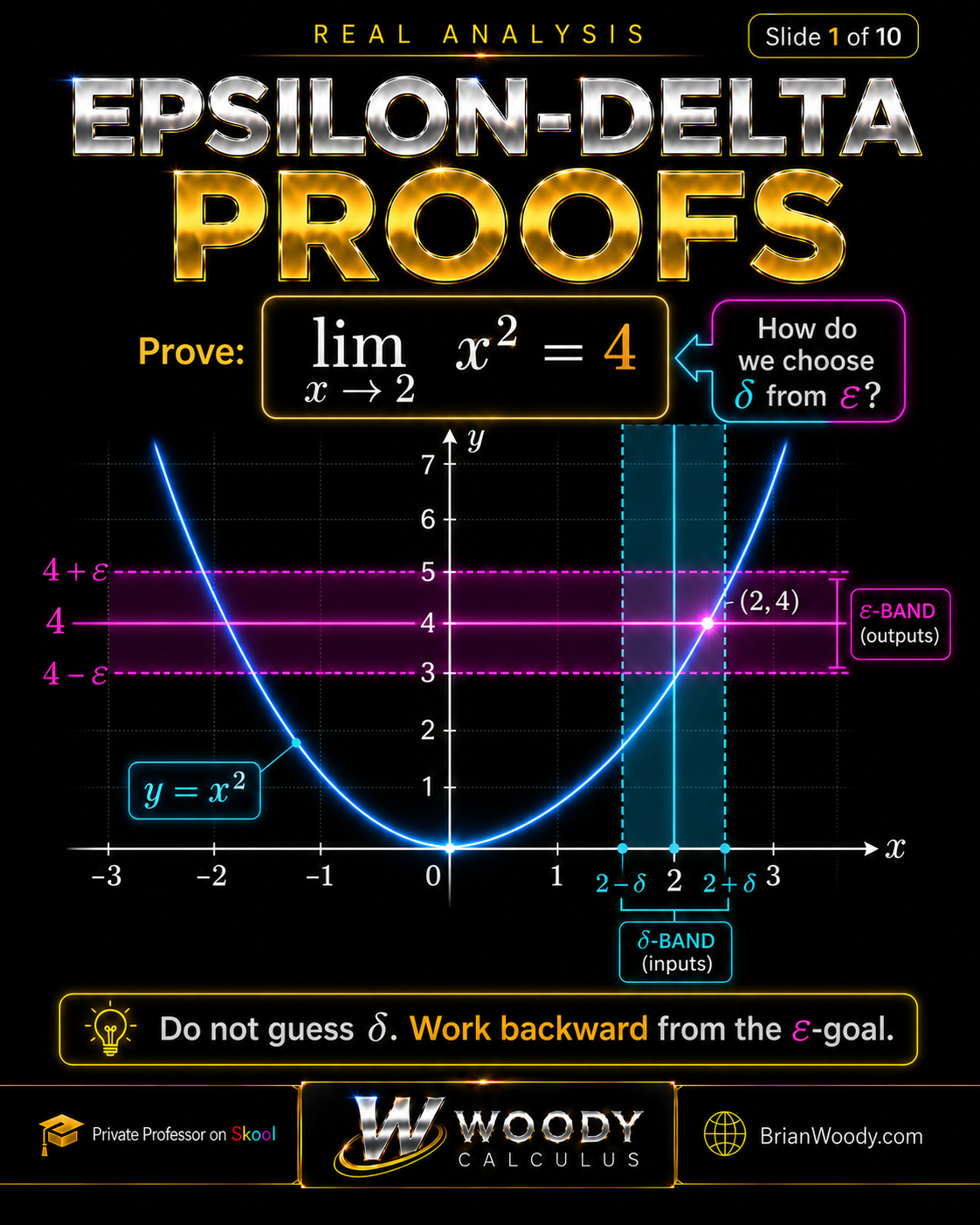
An epsilon-delta proof is the formal way to prove a limit in real analysis: for every output tolerance \(\varepsilon>0\), you must produce an input tolerance \(\delta>0\) that forces the function values into the required target band. For the classic example
\(\lim_{x\to 2}x^2=4\), the clean strategy is to start with the output error \(|x^2-4|\), factor it, locally bound the extra factor, and then choose
\(\delta=\min\!\left(1,\frac{\varepsilon}{5}\right)\).
Plain-language answer:
do not guess \(\delta\). Start with the \(\varepsilon\)-goal, expose the factor controlled by the input distance, build a local bound on everything else, and choose one \(\delta\) that satisfies every condition.
What should you know before learning epsilon-delta proofs?
You should be comfortable with factoring, absolute-value inequalities, function notation, and the informal meaning of a limit.
- Factoring expressions such as \(x^2-4=(x-2)(x+2)\)
- Converting \(|x-2|<1\) into the interval \(1<x<3\)
- Understanding what it means for \(x\) to approach a point \(a\)
- Following a proof line by line without reversing an implication
Quick Summary: Epsilon-Delta Proofs
To prove \(\lim_{x\to 2}x^2=4\), rewrite \(|x^2-4|\) as \(|x-2||x+2|\), use \(|x-2|<1\) to obtain \(|x+2|<5\), and choose \(\delta=\min\!\left(1,\frac{\varepsilon}{5}\right)\).
- Start with the output error, not with a random formula for \(\delta\).
- Factor until the controlled quantity \(|x-2|\) appears.
- Use a local restriction to bound the extra factor \(|x+2|\).
- Take the minimum of the local-bound condition and the \(\varepsilon\)-condition.
- State the proof in the forward direction after discovering \(\delta\) by working backward.
Key Facts
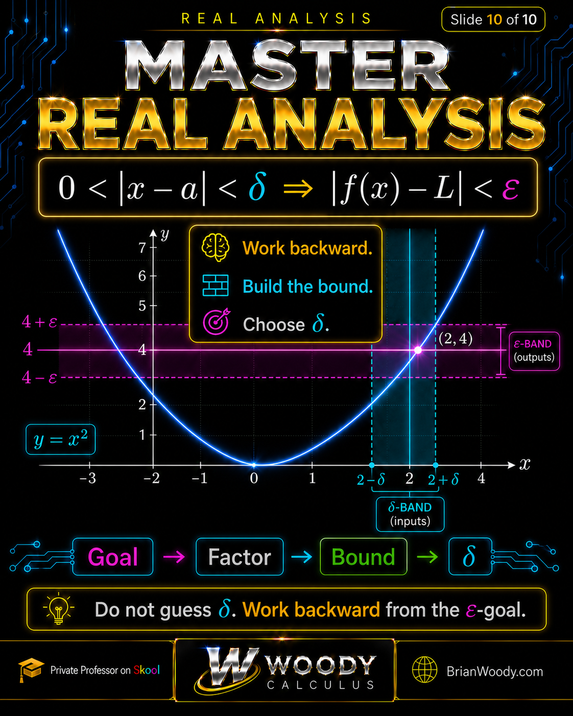
- Formal target: for every \(\varepsilon>0\), find \(\delta>0\) such that \(0<|x-2|<\delta\Rightarrow |x^2-4|<\varepsilon\).
- Main algebra step: \(|x^2-4|=|x-2||x+2|\).
- Local bound: if \(|x-2|<1\), then \(|x+2|<5\).
- Working choice: \(\delta=\min\!\left(1,\frac{\varepsilon}{5}\right)\).
- Proof-writing distinction: discover \(\delta\) backward, but present the proof forward.
- Important nuance: a valid \(\delta\) need not be unique or optimal.
What is the epsilon-delta definition of a limit?
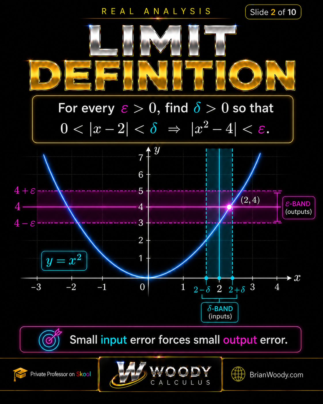
The statement \(\lim_{x\to a}f(x)=L\) means that every requested output accuracy \(\varepsilon>0\) can be guaranteed by restricting the input to a sufficiently small punctured interval \(0<|x-a|<\delta\).
Formal Definition
We say that
\lim_{x\to a}f(x)=L
\]
if for every \(\varepsilon>0\), there exists \(\delta>0\) such that
0<|x-a|<\delta
\quad\Longrightarrow\quad
|f(x)-L|<\varepsilon.
\]
For this lesson,
\(f(x)=x^2\), \(a=2\), and \(L=4\). Therefore, the exact statement to prove is
\text{For every }\varepsilon>0,\text{ there exists }\delta>0\text{ such that }
0<|x-2|<\delta
\quad\Longrightarrow\quad
|x^2-4|<\varepsilon.
\]
Plain-language answer:
no matter how thin the horizontal output band around 4 becomes, there must be some vertical input band around 2 that keeps the graph inside it.
What do \(\varepsilon\) and \(\delta\) mean?
\(\varepsilon\) measures the allowed output error, while \(\delta\) measures the input distance that guarantees that output accuracy.
| Symbol | Meaning | Role in this proof |
|---|---|---|
| \(\varepsilon\) | The output tolerance | We must force \(|x^2-4|<\varepsilon\). |
| \(\delta\) | The input tolerance | We choose \(\delta\) so that \(0<|x-2|<\delta\) is strong enough. |
| \(a\) | The point being approached | Here, \(a=2\). |
| \(L\) | The claimed limit value | Here, \(L=4\). |
| \(|x-a|\) | Input distance | Here, it is \(|x-2|\), the quantity controlled by \(\delta\). |
| \(|f(x)-L|\) | Output error | Here, it is \(|x^2-4|\), the quantity that must be less than \(\varepsilon\). |
The condition \(0<|x-a|\) excludes the point \(x=a\) itself. A limit describes nearby behavior, so the value \(f(a)\) may be different from \(L\) or may not exist at all.
How do you start an epsilon-delta proof?
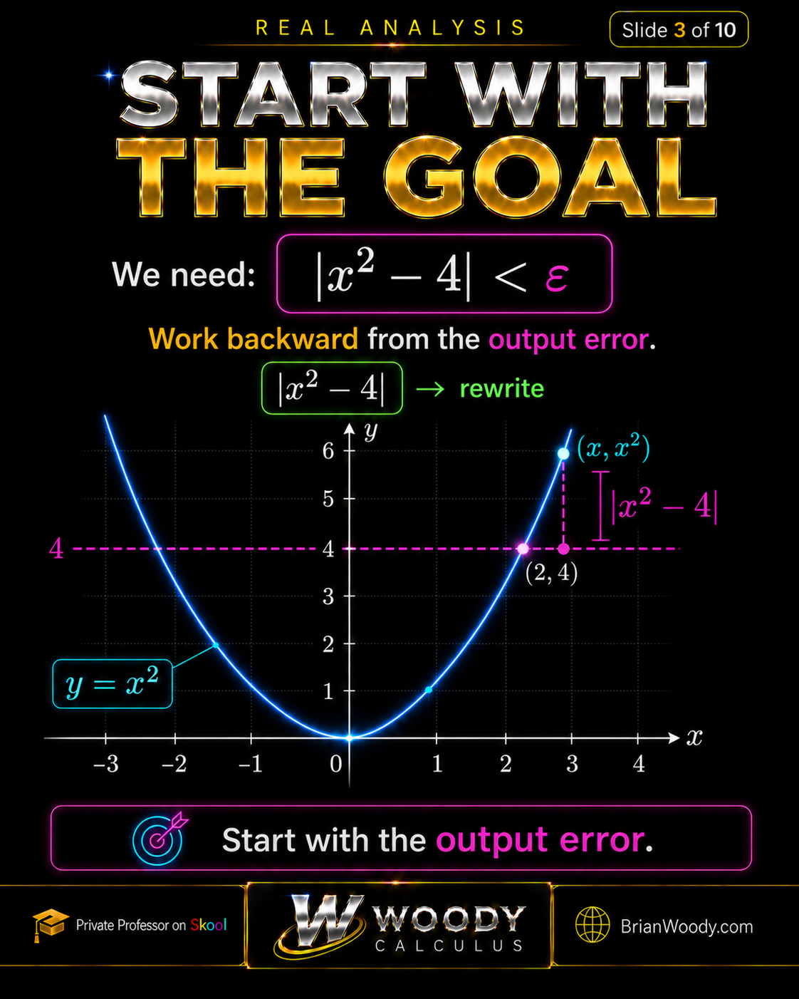
Start with the output error \(|f(x)-L|\), because the algebra of that expression tells you what \(\delta\) must control.
For this problem, the target is
|x^2-4|<\varepsilon.
\]
During scratch work, reason backward from this inequality. During the final proof, begin with \(0<|x-2|<\delta\) and reason forward to the target. This distinction prevents circular arguments.
Plain-language answer:
discovery runs backward; proof presentation runs forward.
How do you rewrite \(|x^2-4|\)?
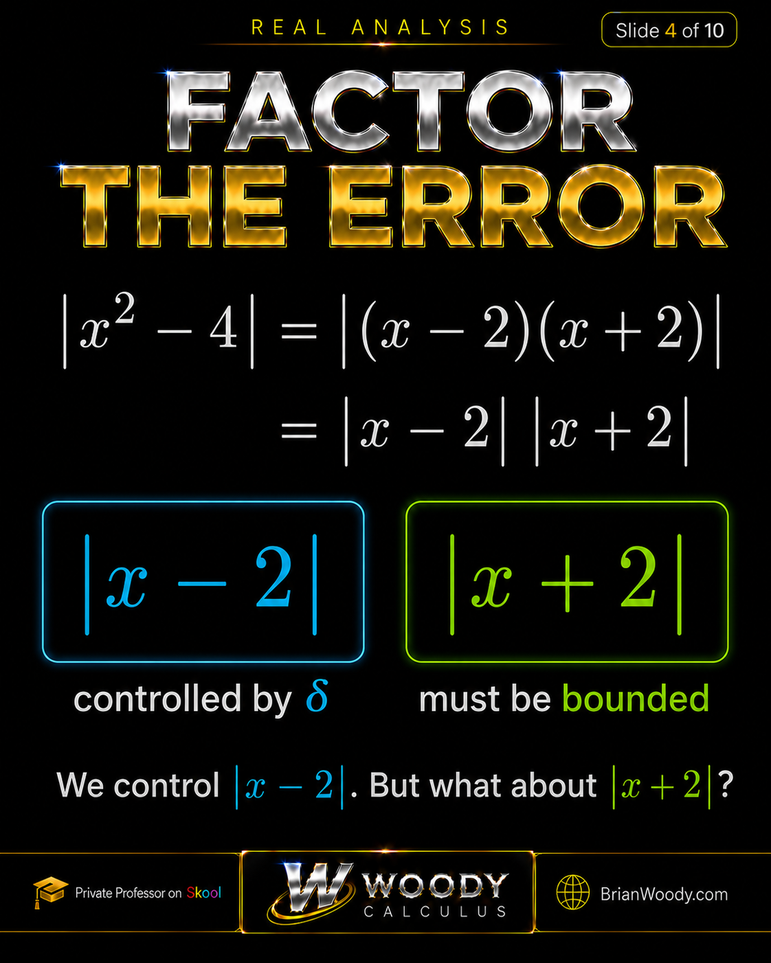
Factor the difference of squares so that the input-distance factor \(|x-2|\) appears explicitly.
|x^2-4|
=|(x-2)(x+2)|
=|x-2|\,|x+2|.
\]
This is the key algebraic move. The definition directly controls \(|x-2|\). The remaining factor \(|x+2|\) is not automatically small, but it does remain bounded when \(x\) is restricted to a sufficiently small neighborhood of 2.
Necessary distinction
We do not need \(|x+2|\) to approach zero. We only need a fixed upper bound for it near \(x=2\).
How do you bound the extra factor \(|x+2|\)?
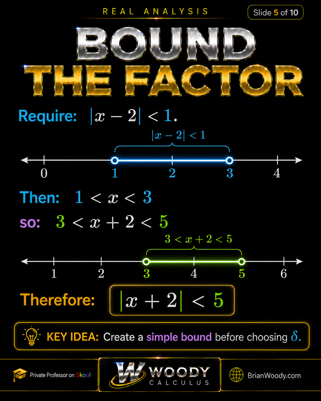
Impose the simple local restriction \(|x-2|<1\), which traps \(x\) between 1 and 3 and therefore forces \(|x+2|<5\).
Require
|x-2|<1.
\]
By the definition of absolute value,
-1<x-2<1.
\]
Adding 2 throughout gives
1<x<3.
\]
Adding 2 again gives
3<x+2<5.
\]
Because \(x+2\) is positive in this interval,
|x+2|=x+2<5.
\]
Plain-language answer:
once \(x\) is kept within one unit of 2, the extra factor can never reach 5.
How do you choose \(\delta\) from \(\varepsilon\)?
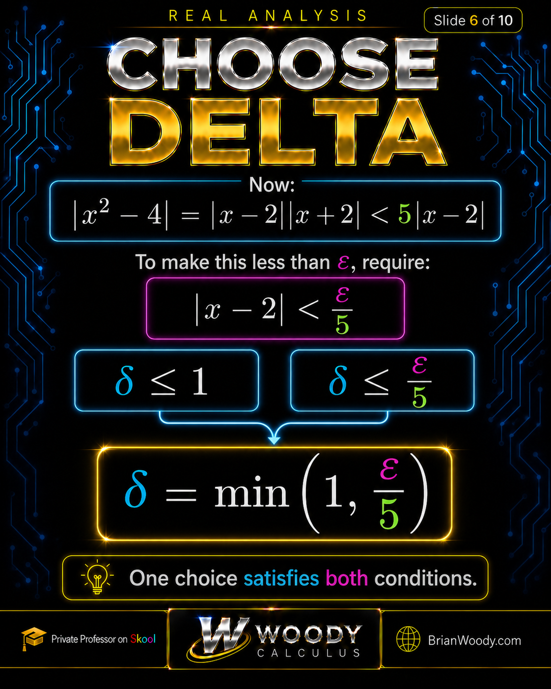
Choose \(\delta\) small enough to preserve the local bound and small enough to make the final estimate less than \(\varepsilon\).
Once \(|x+2|<5\), we have
|x^2-4|=|x-2||x+2|<5|x-2|.
\]
Therefore, it is enough to require
5|x-2|<\varepsilon,
\]
which will follow if
|x-2|<\frac{\varepsilon}{5}.
\]
| Condition | What it controls | Why it is needed |
|---|---|---|
| \(\delta\le 1\) | The local window around 2 | It guarantees \(|x+2|<5\). |
| \(\delta\le \varepsilon/5\) | The final output estimate | It guarantees \(5|x-2|<\varepsilon\). |
| \(\delta=\min(1,\varepsilon/5)\) | Both requirements at once | The minimum is no larger than either permitted upper bound. |
The standard clean choice is
\boxed{\delta=\min\!\left(1,\frac{\varepsilon}{5}\right)}.
\]
Formula memorization is required, but the problem’s structure chooses the formula.
What does the complete epsilon-delta proof look like?
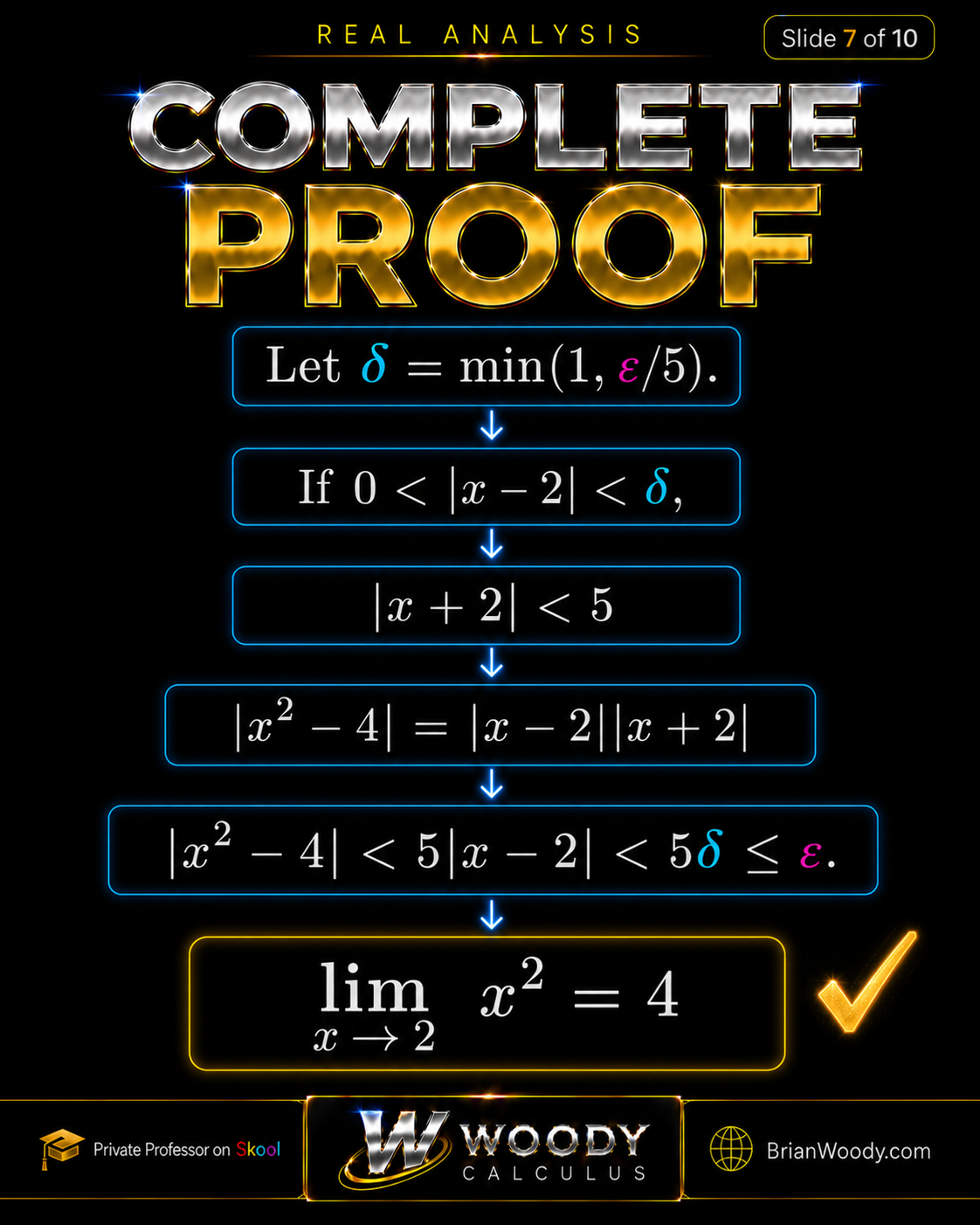
A complete proof states the chosen \(\delta\), assumes \(0<|x-2|<\delta\), and derives \(|x^2-4|<\varepsilon\) without using any unproved step.
Plain-language answer:
the same \(\delta\) keeps \(x\) close enough to 2 to control \(|x+2|\) and close enough to make \(5|x-2|\) smaller than \(\varepsilon\).
How can you independently verify the epsilon-delta proof?
Choose a concrete value of \(\varepsilon\), compute the prescribed \(\delta\), and verify that the proof’s estimate still produces a strict inequality.
Why do we use \(\delta=\min(1,\varepsilon/5)\)?
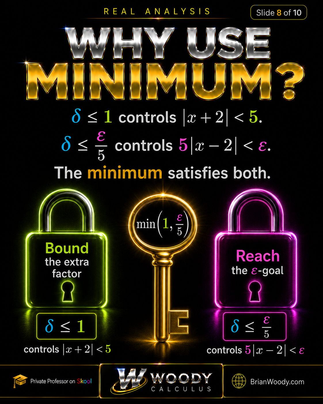
The minimum is used because the proof has two upper-bound requirements, and one number must satisfy both.
- \(\delta\le1\) guarantees the local estimate \(|x+2|<5\).
- \(\delta\le\varepsilon/5\) guarantees the final estimate \(5|x-2|<\varepsilon\).
- The minimum is less than or equal to both allowed upper bounds.
Valid does not mean unique or optimal
The choice \(\delta=\min(1,\varepsilon/5)\) is convenient and sufficient, but it is not the only possible choice. Any smaller positive \(\delta\) also works. In a limit proof, the objective is normally to produce a correct dependence on \(\varepsilon\), not to maximize the size of the input interval.
What is the standard epsilon-delta workflow?
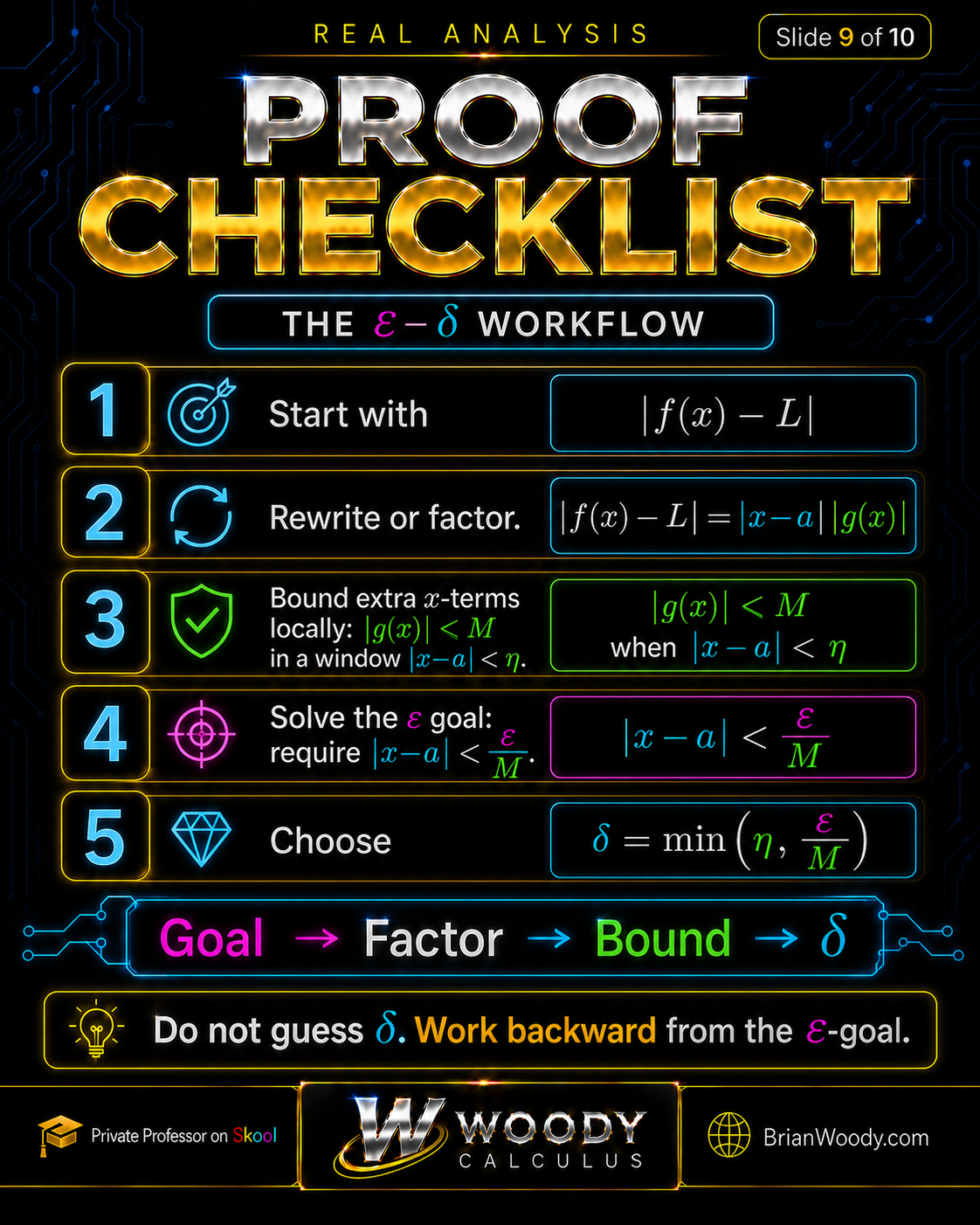
For many algebraic limits, use the sequence: state the goal, rewrite the error, build a local bound, solve the \(\varepsilon\)-condition, and choose \(\delta\).
| Step | What you do | Why it matters |
|---|---|---|
| 1. Start with the goal | Write \(|f(x)-L|\). | This identifies the exact output error that must be controlled. |
| 2. Rewrite or factor | Expose a factor or expression involving \(|x-a|\). | The definition directly controls the input distance. |
| 3. Build a local bound | Restrict \(x\) to a window such as \(|x-a|<\eta\). | This keeps the remaining expression below a fixed constant \(M\). |
| 4. Solve the epsilon-goal | Require \(|x-a|<\varepsilon/M\). | This converts the local bound into the desired output estimate. |
| 5. Choose delta | Take \(\delta=\min(\eta,\varepsilon/M)\). | One choice now satisfies every required upper bound. |
| 6. Write the proof forward | Assume \(0<|x-a|<\delta\) and derive \(|f(x)-L|<\varepsilon\). | This produces a logically valid proof rather than backward scratch work. |
This is a powerful template, but it is not a rigid universal formula. Not every proof literally factors as
\(|f(x)-L|=|x-a||g(x)|\). The deeper strategy is to isolate what the input distance controls and place a justified local bound on what remains.
How does this proof generalize to \(\lim_{x\to a}x^2=a^2\)?
For every real \(a\), the same factor-and-bound method proves \(\lim_{x\to a}x^2=a^2\) with \(\delta=\min\!\left(1,\frac{\varepsilon}{2|a|+1}\right)\).
Plain-language answer:
the original proof is not an isolated trick. It is the \(a=2\) case of a formula that works for the square function at every real number.
What is another example of an epsilon-delta proof?
To prove \(\lim_{x\to3}x^2=9\), a clean choice is \(\delta=\min\!\left(1,\frac{\varepsilon}{7}\right)\).
Worked Micro-Example: Prove \(\lim_{x\to3}x^2=9\)
Start with
|x^2-9|=|x-3||x+3|.
\]
If \(|x-3|<1\), then \(2<x<4\), so \(5<x+3<7\), and therefore \(|x+3|<7\). Choose
\delta=\min\!\left(1,\frac{\varepsilon}{7}\right).
\]
Then \(0<|x-3|<\delta\) implies
|x^2-9|
=|x-3||x+3|
<7|x-3|
<7\delta
\le\varepsilon.
\]
Hence,
\boxed{\lim_{x\to3}x^2=9}.
\]
Try the pattern yourself
Prove \(\lim_{x\to1}x^2=1\). Using the general formula with \(a=1\), one convenient choice is
\delta=\min\!\left(1,\frac{\varepsilon}{3}\right).
\]
What mistakes do students make in epsilon-delta proofs?
Most errors come from guessing \(\delta\), skipping the local bound, reversing the logic, or confusing the limit with the function value at the point.
Mistake: Guessing \(\delta\) immediately
Symptom: The proof begins with \(\delta=\varepsilon\) or \(\delta=\varepsilon/5\) without a derivation.
Cause: The student starts with the unknown input tolerance instead of the output expression that must be controlled.
Fix: Start with \(|f(x)-L|\), rewrite it, and let the algebra determine the necessary restrictions.
Mistake: Forgetting to bound the extra factor
Symptom: The work stops after \(|x^2-4|=|x-2||x+2|\).
Cause: The student sees the desired factor \(|x-2|\) but ignores the uncontrolled factor \(|x+2|\).
Fix: Impose \(|x-2|<1\), derive \(|x+2|<5\), and use the bound explicitly.
Mistake: Writing backward scratch work as the final proof
Symptom: The argument starts with \(|x^2-4|<\varepsilon\) and manipulates the desired conclusion as though it were already known.
Cause: Discovery and proof presentation have been confused.
Fix: Use backward work to discover \(\delta\), then rewrite the finished proof forward from \(0<|x-2|<\delta\).
Mistake: Proving only that \(f(2)=4\)
Symptom: The student substitutes \(x=2\) and declares the limit proved.
Cause: A point value has been confused with nearby behavior.
Fix: Use the punctured condition \(0<|x-2|<\delta\), which specifically excludes \(x=2\).
Mistake: Reversing the meaning of the punctured condition
Symptom: The student says that \(0<|x-2|\) allows \(x=2\).
Cause: The strict lower bound has been misread.
Fix: Since \(|x-2|=0\) exactly when \(x=2\), the condition \(0<|x-2|\) requires \(x\ne2\).
Mistake: Treating the workflow as a rigid universal formula
Symptom: The student believes every limit proof must literally factor into \(|x-a||g(x)|\).
Cause: The example has been memorized without understanding the structural principle.
Fix: Isolate the input-distance quantity and justify a bound on the remaining terms; the exact algebra varies by problem.
Mistake: Believing the chosen \(\delta\) must be the largest possible
Symptom: The student spends time optimizing \(\delta\) instead of finishing a valid proof.
Cause: Sufficiency has been confused with optimality.
Fix: Produce one positive \(\delta\) that works for every permitted \(x\). A smaller valid choice is still a complete proof.
Reading is not mastery
Reading a completed solution is not enough. Rebuild the setup from a blank page, say each implication aloud, and rewrite the perfect proof until the structure becomes automatic.
What is the Woody Calculus exam checklist for epsilon-delta proofs?
Classify first. Choose second. Execute third. Verify last.
- State the exact limit claim.
- Write the epsilon-delta definition from memory with the quantifiers in the correct order.
- Identify \(f(x)\), \(a\), and \(L\).
- Start scratch work with \(|f(x)-L|\).
- Rewrite or factor until the input-distance term appears.
- Build a justified local bound on the remaining factor.
- Choose one \(\delta\) that satisfies every condition.
- Write the final proof forward from \(0<|x-a|<\delta\).
- Preserve strict inequalities where the definition requires them.
- End by stating the limit has been proved.
- Verify the choice with a concrete \(\varepsilon\) or an alternate estimate.
- Rebuild the proof from a blank page and say each step aloud.
Formula memorization is required, but the structure chooses the definition. Memorize the quantifiers and the proof format, then let the algebra determine the bound.
How do you master epsilon-delta proofs in real analysis?
Mastery means you can convert an arbitrary \(\varepsilon\)-goal into a justified \(\delta\)-choice and reconstruct the proof without copying.
The complete mastery sequence
- Memorize the formal definition exactly.
- Translate the symbols into input and output error.
- Work backward from the output goal.
- Factor or rewrite to expose the input-distance term.
- Build a local bound on the extra terms.
- Choose the minimum of all required upper bounds.
- Write the proof forward with every implication justified.
- Generalize the method to a nearby problem.
Rewrite the perfect solution until the method becomes automatic. Then change the center, change the function, and prove that the structure—not the memorized numbers—still guides the argument.
Frequently Asked Questions About Epsilon-Delta Proofs
What is an epsilon-delta proof?
An epsilon-delta proof is a formal proof that a limit is true. It shows that for every output tolerance \(\varepsilon>0\), there exists an input tolerance \(\delta>0\) such that \(0<|x-a|<\delta\) implies \(|f(x)-L|<\varepsilon\).
What is an example of an epsilon-delta proof?
A standard example is proving \(\lim_{x\to2}x^2=4\). Factoring gives \(|x^2-4|=|x-2||x+2|\), and the choice \(\delta=\min(1,\varepsilon/5)\) guarantees that \(|x^2-4|<\varepsilon\).
How do you choose \(\delta\) from \(\varepsilon\)?
Do not guess \(\delta\). Start with \(|f(x)-L|\), rewrite or factor it, locally bound any extra terms, and then choose \(\delta\) so the resulting estimate is less than \(\varepsilon\).
Why do we use \(\delta=\min(1,\varepsilon/5)\) in this proof?
We use \(\delta=\min(1,\varepsilon/5)\) because \(\delta\le1\) guarantees \(|x+2|<5\), while \(\delta\le\varepsilon/5\) guarantees \(5|x-2|<\varepsilon\). The minimum satisfies both conditions at once.
Does the chosen \(\delta\) have to be unique?
No. A proof only needs one valid positive choice of \(\delta\). Any smaller positive value also works, so the chosen \(\delta\) does not have to be optimal.
Why is the condition \(0<|x-2|<\delta\) used?
The condition \(0<|x-2|\) excludes the point \(x=2\) itself because a limit describes the behavior of \(f(x)\) for \(x\) near 2, not the value \(f(2)\). This is why a function can have a limit at a point where it is undefined or has a different value.
Does every epsilon-delta proof follow exactly the same algebraic pattern?
No. Many algebraic examples use the workflow goal, rewrite, bound, and choose \(\delta\), but not every proof has the same factorization. The underlying principle is to isolate the quantity controlled by \(|x-a|\) and justify a bound on what remains.
What is the difference between \(\varepsilon\) and \(\delta\)?
\(\varepsilon\) is the allowed output error \(|f(x)-L|\), while \(\delta\) is the input-distance restriction \(|x-a|\) chosen to guarantee that output accuracy.
Need help with proof-based university mathematics?
The
Woody Calculus Mastery Lab
is the required starting point for students who want help with real analysis, advanced calculus, and proof writing.
Limited
private instruction
may be available after Mastery Lab enrollment. It is selective, limited, normally based on weekly sessions, and not guaranteed.
Visit the
contact page
or explore the
university mathematics help hub.
University mathematics help for real analysis and advanced proof courses
MIT mathematics support
Professor-led support for demanding calculus and proof-based university mathematics.
Harvard mathematics support
Build the conceptual and proof-writing foundation required in advanced mathematics.
Stanford mathematics support
Strengthen rigorous reasoning, theorem recognition, and advanced problem solving.
Princeton mathematics support
Targeted help for students moving from computation into proof-based analysis.
UCLA mathematics support
Structured preparation for calculus, real analysis, and proof-oriented coursework.
UCF mathematics support
University-level help with calculus, differential equations, and advanced mathematical preparation.
Reviews and trust
Read
Woody Calculus 5-star Google reviews
and view
Brian M. Woody’s 5.0 RateMyProfessors rating.
Woody Calculus provides university-level mathematical instruction, structured practice, and long-term mastery—not generic tutoring and not a shortcut answer service.