DIFFERENTIAL EQUATIONS · FIRST-ORDER ODEs · VISUAL LESSON
Original Woody Calculus Lesson
How Do You Test and Solve an Exact Differential Equation?
A first-order differential equation \(M(x,y)\,dx+N(x,y)\,dy=0\) is exact on a region when there is a potential function \(F(x,y)\) satisfying \(F_x=M\) and \(F_y=N\). On an open rectangle where the relevant first partial derivatives are continuous, test exactness with \(M_y=N_x\). If the test passes, recover \(F\) and write the implicit solution \(F(x,y)=C\).
Direct answer: An exact equation hides one potential function. On an open rectangle where the relevant first partial derivatives are continuous, compare the y-derivative of M with the x-derivative of N. If they agree throughout the rectangle, integrate one coefficient, use the other to recover the missing one-variable term, set the potential equal to a constant, and verify.
Exact equations turn a differential equation into a reconstruction problem. Instead of separating variables or forcing a linear form, you identify a hidden total differential \(dF\). This lesson develops the test, the recovery algorithm, a complete initial-value problem, special integrating factors, the conservative-field connection, and the domain caveat that makes the theorem fully rigorous.
Key Takeaways
- Test: on a suitable rectangle, \(M_y=N_x\) is equivalent to exactness.
- Recover: integrate one component, add a function of the other variable, and match the remaining partial derivative.
- Verify: write \(F(x,y)=C\), apply any initial condition, and differentiate implicitly to check the result.
Estimated reading time: 35–45 minutes.

What Is an Exact Differential Equation?
Begin with a first-order differential equation written in differential form:
M(x,y)\,dx+N(x,y)\,dy=0.
\]
The equation is exact on a region \(R\) if there is a differentiable scalar function \(F:R\to\mathbb{R}\) such that
F_x(x,y)=M(x,y),\qquad F_y(x,y)=N(x,y).
\]
Because the total differential of \(F\) is
dF=F_x\,dx+F_y\,dy=M\,dx+N\,dy,
\]
the differential equation becomes \(dF=0\). Therefore \(F\) is constant along every solution curve:
\boxed{F(x,y)=C}.
\]

Solution curves are level curves
The answer \(F(x,y)=C\) is usually implicit. Each value of \(C\) selects one level curve of the potential function.
The Exactness Test: When Does \(M_y=N_x\) Work?
EXACTNESS THEOREM
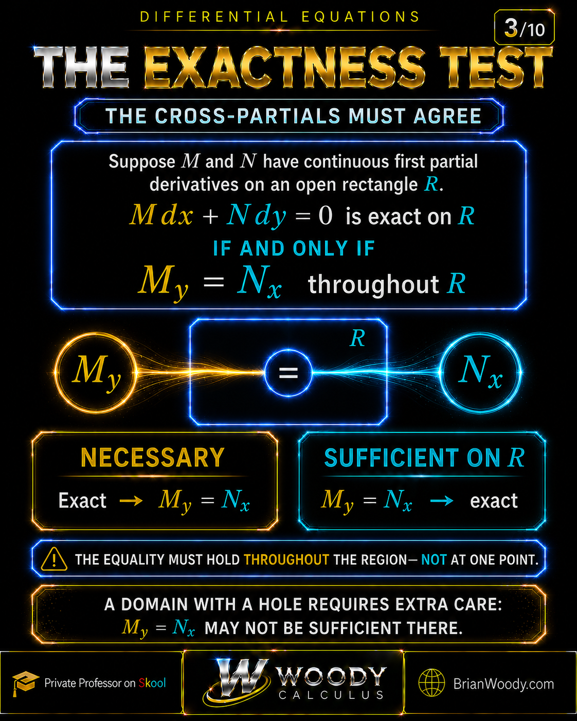
Suppose \(M\) and \(N\) have continuous first partial derivatives on an open rectangle \(R\). Then
M(x,y)\,dx+N(x,y)\,dy=0
\quad\text{is exact on }R
\quad\Longleftrightarrow\quad
M_y=N_x\text{ throughout }R.
\]
Why the condition is necessary: if \(M=F_x\) and \(N=F_y\), then continuity of the relevant second partial derivatives gives
M_y=(F_x)_y=F_{xy}=F_{yx}=(F_y)_x=N_x.
\]
Why the rectangle matters: on an open rectangle, equality of the cross-partials is also sufficient for a globally defined potential function on that rectangle. On a region with a hole, the equality can hold locally everywhere while a single-valued global potential still fails to exist.
| What you know on the region | What you may conclude | Required caution |
|---|---|---|
| Continuous first partials and \(M_y=N_x\) on an open rectangle | The equation is exact there. | Construct \(F\) and verify both partial derivatives. |
| \(M_y\ne N_x\) at even one point | The equation is not exact on any region containing that point. | Classify again or look for a valid integrating factor. |
| \(M_y=N_x\) only at one point | No regional conclusion follows. | The equality must hold throughout the region. |
| \(M_y=N_x\) on a domain with a hole | The form is locally exact. | Global exactness needs a domain argument. |
Do not test at one point
Exactness is a property on a region. Compute \(M_y\) and \(N_x\) as functions and compare them throughout the intended domain.
How to Recover the Potential Function \(F(x,y)\)
Once the equation passes the exactness test, reconstruct \(F\). The following five steps are the complete solution algorithm.
-
1
Identify M and N
Write the equation as \(M(x,y)\,dx+N(x,y)\,dy=0\), preserving the order of \(dx\) and \(dy\).
-
2
Test exactness on the region
Compute \(M_y\) and \(N_x\). On a suitable rectangle, continue only when \(M_y=N_x\).
-
3
Integrate one component
Integrate \(M\) with respect to \(x\): \(F(x,y)=\int M(x,y)\,dx+g(y)\).
-
4
Match the other component
Differentiate the result with respect to \(y\), set \(F_y=N\), and solve for \(g^{\prime}(y)\).
-
5
Write and verify the solution
Integrate \(g^{\prime}\), write \(F(x,y)=C\), apply any initial condition, and check \(F_x=M\) and \(F_y=N\).
\(F=\int M\,dx+g(y)\)
\(F=\int N\,dy+h(x)\)

Why does \(g^{\prime}(y)\) come out independent of \(x\)?
Let \(A(x,y)=\int M(x,y)\,dx\). Matching gives \(g^{\prime}(y)=N-A_y\). Differentiate the right-hand side with respect to \(x\):
\frac{\partial}{\partial x}\bigl(N-A_y\bigr)=N_x-A_{yx}=N_x-M_y=0.
\]
Exactness is precisely what forces the remaining expression to depend only on \(y\). The recovery method is a theorem, not a memorized trick.
Worked Example: Solve an Exact Differential Equation
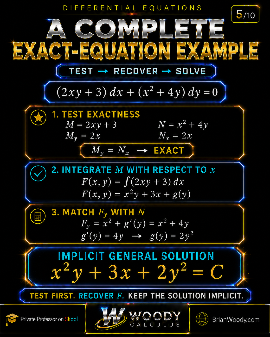
Solve
(2xy+3)\,dx+(x^2+4y)\,dy=0.
\]
Step 1: Identify and test
M(x,y)=2xy+3,\qquad N(x,y)=x^2+4y.
\]
\[
M_y=2x,\qquad N_x=2x.
\]
The first partial derivatives are continuous on \(\mathbb{R}^2\), and \(M_y=N_x\) everywhere. The equation is exact on \(\mathbb{R}^2\).
Step 2: Integrate \(M\) with respect to \(x\)
F(x,y)=\int(2xy+3)\,dx=x^2y+3x+g(y).
\]
The integration is with respect to \(x\), so \(y\) is held constant. The missing integration term may be any function of \(y\).
Step 3: Match \(F_y\) with \(N\)
F_y=x^2+g^{\prime}(y)=N=x^2+4y.
\]
\[
g^{\prime}(y)=4y\qquad\Longrightarrow\qquad g(y)=2y^2.
\]
Step 4: Write the implicit solution
\boxed{x^2y+3x+2y^2=C}.
\]
Exact Differential Equation Initial-Value Problem
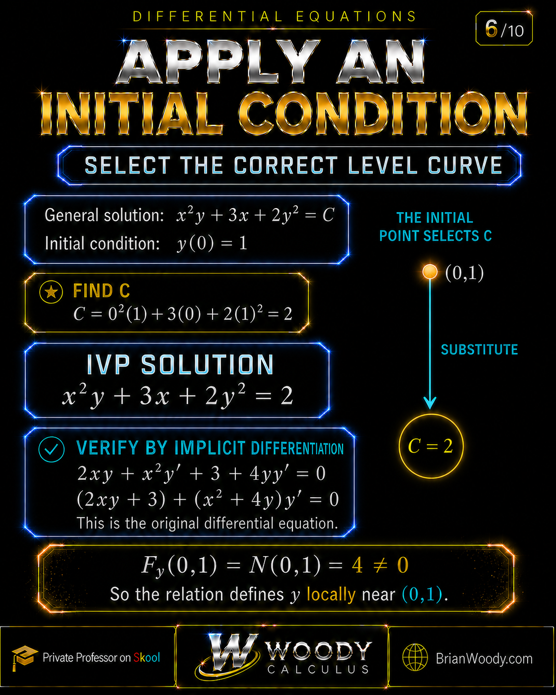
Now impose the initial condition \(y(0)=1\) on the solution family
x^2y+3x+2y^2=C.
\]
Substitute \((x,y)=(0,1)\):
C=0^2(1)+3(0)+2(1)^2=2.
\]
\boxed{x^2y+3x+2y^2=2}.
\]
Verify by implicit differentiation
\frac{d}{dx}\bigl(x^2y+3x+2y^2\bigr)=0,
\]
\[
2xy+x^2y^{\prime}+3+4yy^{\prime}=0,
\]
\[
(2xy+3)+(x^2+4y)y^{\prime}=0.
\]
This is exactly the original differential equation after dividing its differential form by \(dx\).
Does the implicit relation define \(y\) as a function of \(x\)?
Here \(F_y=x^2+4y\), so
F_y(0,1)=4\ne0.
\]
By the implicit function theorem, the level curve \(F(x,y)=2\) defines a unique differentiable function \(y=y(x)\) locally near \((0,1)\).
What If the Differential Equation Is Not Exact?
Consider
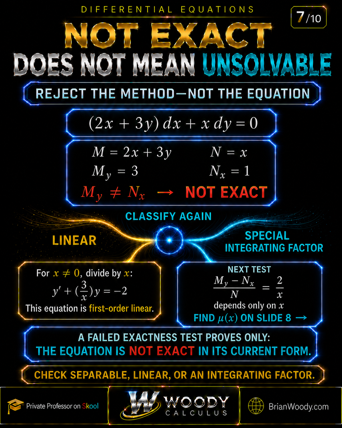
(2x+3y)\,dx+x\,dy=0.
\]
Here
M=2x+3y,\qquad N=x,
\]
\[
M_y=3,\qquad N_x=1.
\]
Because \(M_y\ne N_x\), the equation is not exact as written. That conclusion does not mean the ODE has no solution. It means the exact-equation method does not yet apply.
Classify before choosing a method
For \(x\ne0\), divide the equation by \(dx\) and then by \(x\):
(2x+3y)+xy^{\prime}=0,
\]
\[
y^{\prime}+\frac{3}{x}y=-2.
\]
This is also a first-order linear equation on any interval that does not cross \(x=0\). Classification reveals available methods; it does not force one method.
“Not exact” is not “unsolvable”
A nonexact equation may be separable, linear, homogeneous, Bernoulli, or convertible to exact form. The failed test identifies the current form, not the existence of solutions.
Special Integrating Factors for Nonexact Equations
For a general nonexact equation, finding an integrating factor can be difficult. Two important special tests produce an integrating factor depending on only one variable.
If \(\dfrac{M_y-N_x}{N}=f(x)\), then \(\mu(x)=e^{\int f(x)\,dx}\).
If \(\dfrac{N_x-M_y}{M}=g(y)\), then \(\mu(y)=e^{\int g(y)\,dy}\).
Apply the \(\mu(x)\) test
For \(M=2x+3y\) and \(N=x\),
\frac{M_y-N_x}{N}=\frac{3-1}{x}=\frac{2}{x},
\]
which depends only on \(x\). Therefore, on either interval \(x>0\) or \(x<0\),
\mu(x)=e^{\int 2/x\,dx}=e^{2\ln|x|}=x^2.
\]
Multiply the entire differential equation by \(x^2\):
(2x^3+3x^2y)\,dx+x^3\,dy=0.
\]
The transformed coefficients satisfy
\frac{\partial}{\partial y}(2x^3+3x^2y)=3x^2
=\frac{\partial}{\partial x}(x^3),
\]
so the transformed equation is exact. Recover the potential:
F=\int(2x^3+3x^2y)\,dx
=\frac12x^4+x^3y+g(y).
\]
\[
F_y=x^3+g^{\prime}(y)=x^3
\quad\Longrightarrow\quad g^{\prime}(y)=0.
\]
\boxed{\frac12x^4+x^3y=C},\qquad x>0\text{ or }x<0.
\]

Why the interval restriction matters
The ratio \(2/x\) and the linear standard form are undefined at \(x=0\). Moreover, multiplying by \(\mu=x^2\) is reversible only where \(\mu\ne0\). Work on \(x>0\) or \(x<0\), and never silently cross the singular line.
An advanced solution-family detail
When \(C=0\), the transformed relation factors as \(x^3(x/2+y)=0\). On \(x\ne0\), it gives \(y=-x/2\). Substitution into the original differential equation shows that this particular function satisfies \((2x+3y)+xy^{\prime}=0\) for every real \(x\), including \(x=0\). The method still had to exclude \(x=0\) because its division and integrating-factor steps were not valid there.
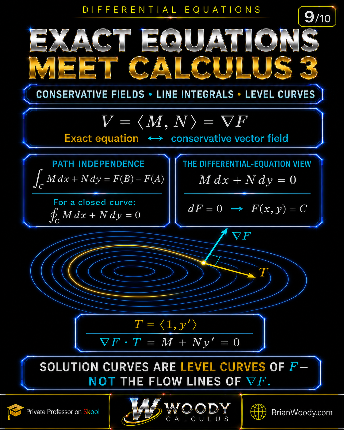
Exact Differential Equations and Conservative Vector Fields
Associate the differential equation with the vector field
\mathbf{V}(x,y)=\langle M(x,y),N(x,y)\rangle.
\]
If the equation is exact, then \(\mathbf{V}=\nabla F\). Thus the vector field is conservative, its line integrals are path independent on the appropriate domain, and every closed-curve integral is zero:
\int_C M\,dx+N\,dy=F(B)-F(A),
\]
\[
\oint_C M\,dx+N\,dy=0.
\]
Why the ODE solution follows a level curve
If a solution is written locally as \(y=y(x)\), a tangent vector is \(\mathbf{T}=\langle1,y^{\prime}\rangle\). Along a solution,
\nabla F\cdot\mathbf{T}
=\langle M,N\rangle\cdot\langle1,y^{\prime}\rangle
=M+Ny^{\prime}=0.
\]
Therefore the gradient is perpendicular to the solution curve. The solution curves are level curves of \(F\), not flow lines of \(\nabla F\).
The Domain-with-a-Hole Counterexample
The equality \(M_y=N_x\) does not by itself guarantee a single global potential on every possible domain. On the punctured plane \(D=\mathbb{R}^2\setminus\{(0,0)\}\), consider
M(x,y)=-\frac{y}{x^2+y^2},\qquad
N(x,y)=\frac{x}{x^2+y^2}.
\]
A direct computation gives
M_y=\frac{y^2-x^2}{(x^2+y^2)^2}
=N_x
\]
at every point of \(D\). However, parametrize the unit circle counterclockwise by \(x=\cos t\), \(y=\sin t\), \(0\le t\le2\pi\). Then \(dx=-\sin t\,dt\), \(dy=\cos t\,dt\), and
\oint_C M\,dx+N\,dy
=\int_0^{2\pi}\bigl(\sin^2 t+\cos^2 t\bigr)\,dt
=2\pi\ne0.
\]
A globally exact form would have zero integral around every closed curve. Therefore this form is not globally exact on the punctured plane, even though \(M_y=N_x\) there. It is exact on smaller simply connected regions that do not wrap around the origin.
Introductory-course rule
When your textbook states the test on an open rectangle, the topological difficulty disappears. Use the rectangle hypothesis exactly as stated; mention simply connected domains only when the course expects the broader theorem.
Exact Differential Equations Decision Map
Use this four-part map to classify the equation, test exactness on the correct region, recover a potential when possible, and verify the final result.
Recognize: write the ODE as \(M\,dx+N\,dy=0\) and identify the intended region.
Test: compute \(M_y\) and \(N_x\) throughout that region.
Recover: if exact, integrate one component and match the other; if not exact, reclassify or test a special integrating factor.
Verify: write \(F=C\), apply initial data, respect the domain, and differentiate to check the result.

Common Exact Differential Equation Mistakes
Most errors come from testing the wrong derivatives, omitting the missing one-variable function, or losing a domain restriction introduced during reclassification.
Swapping the derivatives
The standard comparison is \(M_y\) with \(N_x\), not \(M_x\) with \(N_y\).
Testing only at one point
Exactness must hold throughout the region where the potential is claimed.
Forgetting \(g(y)\) or \(h(x)\)
When integrating in one variable, the integration “constant” may depend on the other variable.
Integrating both terms and adding
That usually double-counts shared terms. Integrate one component, then use the other to match.
Stopping after \(M_y=N_x\)
The test proves exactness; it does not yet produce the solution. You must recover \(F\).
Ignoring the integrating-factor sign
The \(\mu(x)\) and \(\mu(y)\) ratios have opposite numerator order. Re-derive or check them carefully.
Dropping the domain restriction
Division and integrating factors may require an interval on which denominators and multipliers are nonzero.
Confusing level curves with flow lines
The vector field \(\nabla F\) is normal to \(F=C\); it does not run tangent to the ODE solution.
Exact Differential Equations Mastery Check
Try each problem before opening the solution. The set covers exactness, potential recovery, an initial-value problem, a \(\mu(y)\) integrating factor, and the domain-with-a-hole caveat.
1. Solve \((3x^2+2y)\,dx+(2x+4y^3)\,dy=0\).
Solution
\(M_y=2=N_x\), so the equation is exact on \(\mathbb{R}^2\). Integrate \(M\) in \(x\):
Then \(F_y=2x+g^{\prime}(y)=2x+4y^3\), so \(g^{\prime}(y)=4y^3\) and \(g(y)=y^4\). Therefore
2. Apply \(y(0)=1\) to the solution in Problem 1.
Solution
Substitute \((0,1)\): \(C=0+0+1=1\). The IVP solution is
Also, \(F_y(0,1)=2(0)+4(1)^3=4\ne0\), so the relation defines \(y\) locally as a function of \(x\) near the initial point.
3. Is \((y\cos x+2x)\,dx+(\sin x+2y)\,dy=0\) exact? Solve it.
Solution
\(M_y=\cos x=N_x\), so the equation is exact on \(\mathbb{R}^2\). Integrating \(M\) in \(x\) gives
Then \(F_y=\sin x+g^{\prime}(y)=\sin x+2y\), so \(g(y)=y^2\). Thus
4. Test \((e^x\cos y)\,dx-(e^x\sin y)\,dy=0\) and solve.
Solution
\(M_y=-e^x\sin y=N_x\), so the equation is exact. Since
matching \(F_y=-e^x\sin y+g^{\prime}(y)\) with \(N=-e^x\sin y\) gives \(g^{\prime}(y)=0\). Therefore
5. Use an integrating factor depending only on \(y\) to solve \(y\,dx+2x\,dy=0\) on \(y>0\).
Solution
Here \(M=y\) and \(N=2x\), so \(M_y=1\ne2=N_x\). The equation is not exact as written. However,
which depends only on \(y\). On \(y>0\),
Multiplying by \(y\), which is nonzero on the chosen domain, gives
The transformed equation is exact because \((y^2)_y=2y=(2xy)_x\). Integrating \(y^2\) with respect to \(x\) gives \(F=xy^2\), so
6. Why does \(M_y=N_x\) not prove global exactness on every domain?
Solution
The equality is a local differential condition. A domain with a hole may contain closed curves around the hole for which the line integral is nonzero. The punctured-plane form \(-y/(x^2+y^2)\,dx+x/(x^2+y^2)\,dy\) has equal cross-partials but integral \(2\pi\) around the unit circle, so it has no single-valued global potential on the punctured plane.
Exact Differential Equations Glossary
These definitions connect the computational method with its geometric and domain-level meaning.
- Exact differential equation
- An equation \(M\,dx+N\,dy=0\) for which \(M=F_x\) and \(N=F_y\) on the stated region.
- Potential function
- A scalar function \(F(x,y)\) whose gradient is \(\langle M,N\rangle\); exact-equation solutions are \(F=C\).
- Total differential
- The expression \(dF=F_x\,dx+F_y\,dy\), which records the first-order change in \(F\).
- Exactness test
- On a suitable rectangle, the comparison \(M_y=N_x\) used to determine whether \(M\,dx+N\,dy\) is exact.
- Integrating factor
- A nonzero multiplier \(\mu\) that transforms a differential equation into exact form on a chosen domain.
- Conservative vector field
- A vector field that is the gradient of a scalar potential; its line integrals are path independent on the appropriate domain.
- Level curve
- A curve \(F(x,y)=C\) along which the potential is constant.
- Simply connected region
- Informally, a connected region without holes; under standard smoothness assumptions, this removes the global obstruction in the cross-partial test.
- Implicit solution
- A relation \(F(x,y)=C\) that describes solution curves without necessarily solving explicitly for \(y\).
- Initial-value problem
- A differential equation together with a condition such as \(y(x_0)=y_0\), which selects a particular constant \(C\).
Frequently Asked Questions About Exact Differential Equations
These concise answers summarize the test, the recovery method, integrating factors, verification, and the global-domain limitation.
What is an exact differential equation?
An equation \(M(x,y)\,dx+N(x,y)\,dy=0\) is exact on a region if there is a potential function \(F(x,y)\) such that \(F_x=M\) and \(F_y=N\). Its implicit solutions are the level curves \(F(x,y)=C\).
How do you test whether a differential equation is exact?
On an open rectangle where \(M\) and \(N\) have continuous first partial derivatives, compute \(M_y\) and \(N_x\). The equation is exact on that rectangle if and only if \(M_y=N_x\) throughout it.
How do you find the potential function F(x,y)?
Integrate \(M\) with respect to \(x\) and add an unknown function \(g(y)\). Differentiate the result with respect to \(y\), set it equal to \(N\), and solve for \(g^{\prime}(y)\). You may instead integrate \(N\) first and add \(h(x)\).
Why do you add g(y) after integrating M with respect to x?
A function of \(y\) is constant with respect to \(x\), so it disappears when differentiated by \(x\). Adding \(g(y)\) restores every term that \(F_x=M\) cannot detect.
What should you do if M_y is not equal to N_x?
The equation is not exact as written. Reclassify it as separable, linear, homogeneous, Bernoulli, or another type, or test whether a valid integrating factor can convert it to exact form.
What are the special integrating factor formulas for exact equations?
If \((M_y-N_x)/N\) depends only on \(x\), then \(\mu(x)=\exp(\int (M_y-N_x)/N\,dx)\). If \((N_x-M_y)/M\) depends only on \(y\), then \(\mu(y)=\exp(\int (N_x-M_y)/M\,dy)\), on domains where the formulas are defined.
Is M_y = N_x always sufficient for exactness?
It is sufficient on an open rectangle and, more generally, under standard smoothness assumptions on a simply connected domain. On a domain with a hole, equal cross-partials may give only local exactness, not a single global potential.
Are exact differential equation solutions explicit or implicit?
They are naturally implicit: \(F(x,y)=C\). You only need to solve explicitly for \(y\) when the problem requests it and the algebra permits it.
How are exact equations related to conservative vector fields?
The coefficient field \(\langle M,N\rangle\) equals \(\nabla F\) when the equation is exact. Consequently, line integrals are path independent on the appropriate domain, and the ODE solutions \(F=C\) are level curves perpendicular to the gradient.
How do you verify an exact differential equation solution?
Differentiate \(F(x,y)=C\) implicitly to obtain \(F_x+F_y y^{\prime}=0\), and confirm that this is \(M+Ny^{\prime}=0\). Also check any initial condition and every domain restriction.
References and Further Study
This lesson follows the standard undergraduate treatment of exact first-order equations and connects it to the vector-calculus theory of conservative fields.
- Dennis G. Zill, A First Course in Differential Equations with Modeling Applications.
- William E. Boyce, Richard C. DiPrima, and Douglas B. Meade, Elementary Differential Equations and Boundary Value Problems.
- Earl A. Coddington, An Introduction to Ordinary Differential Equations.
- Jerrold E. Marsden and Anthony J. Tromba, Vector Calculus.
Continue Learning Differential Equations
Use these related lessons to strengthen method selection, qualitative interpretation, numerical approximation, and the Calculus 3 connection.