DIFFERENTIAL EQUATIONS · INITIAL-VALUE PROBLEMS · VISUAL LESSON
Original Woody Calculus Lesson
Does the Solution Exist—and Is It the Only One?
For the initial-value problem \(y^{\prime}=f(x,y)\), \(y(x_0)=y_0\), continuity of \(f\) on a rectangle containing \((x_0,y_0)\) guarantees at least one local solution. If \(\partial f/\partial y\) is also continuous there, the local solution is unique. These conditions are sufficient, not necessary, and they do not by themselves determine the maximal interval on which the solution exists.
That short statement answers two different questions: existence asks whether any solution curve passes through the prescribed point, while uniqueness asks whether exactly one does. The distinction controls how we interpret initial conditions, slope fields, numerical approximations, nonlinear models, and the possibility that solutions may branch, blow up, or fail to exist.
Key Takeaways
- Local existence: continuity of \(f(x,y)\) near the initial point guarantees at least one local solution.
- Local uniqueness: continuity of both \(f\) and \(\partial f/\partial y\) there guarantees that the local solution is unique.
- Maximal interval: a separate analysis must still check domain restrictions, singularities, and finite-time blow-up.
Estimated reading time: 30–40 minutes.
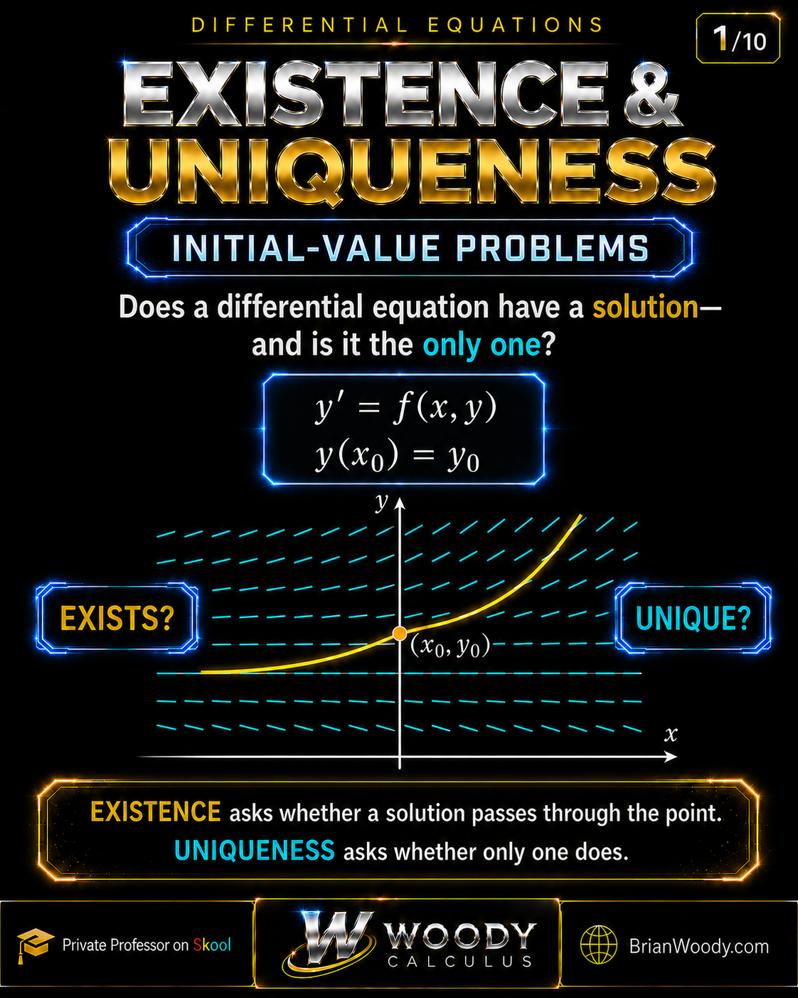
An Initial-Value Problem Has Three Possible Outcomes
An initial-value problem, or IVP, combines a differential equation with data at a specific point:
y^{\prime}=f(x,y), \qquad y(x_0)=y_0.
\]
The initial condition requires the solution graph to pass through \((x_0,y_0)\). Exactly one of the following may occur:
No solution
No classical solution curve satisfies both the differential equation and the prescribed initial condition.
Exactly one solution
A single local solution curve passes through the initial point. The IVP is locally uniquely solvable.
Multiple solutions
Two or more different solution curves satisfy the same differential equation and initial condition.

Existence and uniqueness are separate claims
A theorem may guarantee that at least one solution exists without guaranteeing that the solution is unique. Never combine the two conclusions unless the hypotheses justify both.
Existence and Uniqueness Theorem for First-Order Differential Equations
Let \((x_0,y_0)\) lie inside an open rectangle
R=\left\{(x,y):|x-x_0|<a,\ |y-y_0|<b\right\}.
\]
THEOREM
Local existence
If \(f(x,y)\) is continuous on \(R\), then the IVP
y^{\prime}=f(x,y),\qquad y(x_0)=y_0
\]
has at least one solution on some open interval containing \(x_0\).
Local uniqueness
If both \(f\) and \(\partial f/\partial y\) are continuous on \(R\), then that local solution is unique.
The existence statement is associated with the Peano existence theorem. The additional derivative condition is a standard, easy-to-check sufficient condition for the local Lipschitz hypothesis used by the Picard–Lindelöf theorem. In an introductory course, the practical test is therefore:
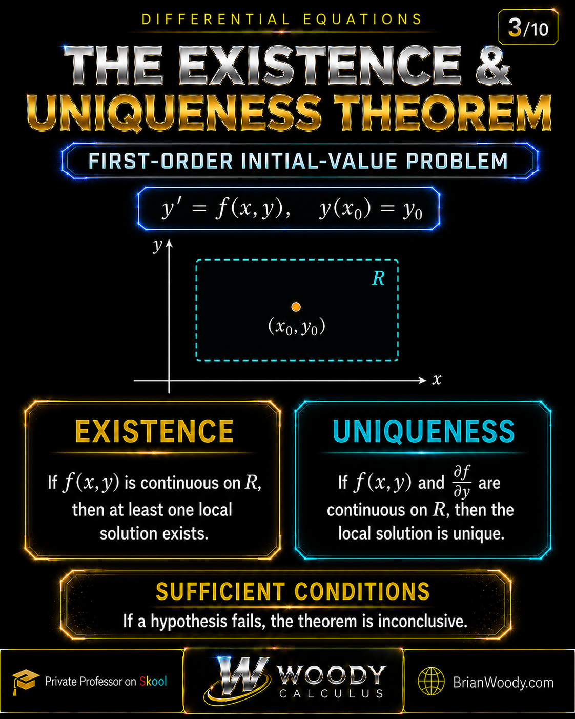
The logical warning that protects your answer
These hypotheses are sufficient. If one fails, the theorem is generally inconclusive. A failed hypothesis does not automatically prove nonexistence or nonuniqueness.
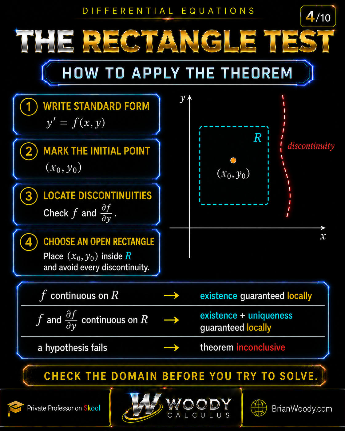
The Four-Step Rectangle Test
The theorem is local, so we do not need \(f\) and \(f_y\) to be continuous everywhere. We need an open rectangle around the initial point that stays inside the region where the required functions are continuous.
- 1
Write the equation in standard form
Solve for \(y^{\prime}\) and identify \(f(x,y)\) in \(y^{\prime}=f(x,y)\).
- 2
Locate the initial point
Translate \(y(x_0)=y_0\) into the point \((x_0,y_0)\).
- 3
Find every relevant discontinuity
Check where \(f\) is undefined or discontinuous. For uniqueness, also check \(f_y=\partial f/\partial y\).
- 4
Choose a valid open rectangle
Place \((x_0,y_0)\) inside a rectangle that avoids those discontinuities, then state only the conclusion supported by the theorem.
| What you verify near \((x_0,y_0)\) | Valid conclusion | What you may not conclude |
|---|---|---|
| \(f\) is continuous | At least one local solution exists. | Uniqueness has not yet been established. |
| \(f\) and \(f_y\) are continuous | Exactly one local solution exists. | Global existence still does not automatically follow. |
| \(f\) is not continuous | The standard existence test is inconclusive. | Do not say “no solution” without a separate argument. |
| \(f_y\) is not continuous | The standard uniqueness test is inconclusive. | Do not say “multiple solutions” without exhibiting or proving them. |
| \(f(x_0,y_0)\) is undefined | No classical solution can satisfy the IVP at that point. | Do not treat a formal curve as a classical solution. |
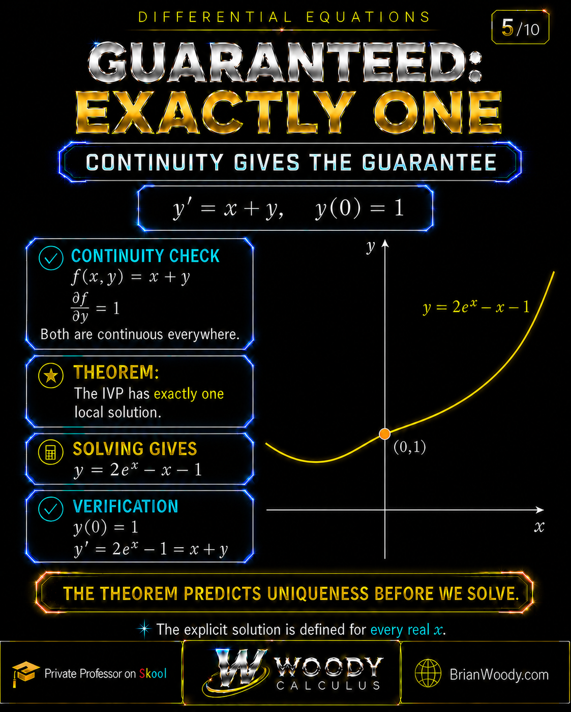
Worked Example: A Unique Solution to \(y^{\prime}=x+y\), \(y(0)=1\)
Start with
Here \(f(x,y)=x+y\), so
Both functions are continuous on all of \(\mathbb{R}^2\). Therefore, the theorem guarantees exactly one local solution through \((0,1)\) before we solve the equation.
Solve with an integrating factor
Rewrite the equation in first-order linear form:
The integrating factor is
Multiplying the equation by \(e^{-x}\) gives
e^{-x}y^{\prime}-e^{-x}y=xe^{-x}
\quad\Longrightarrow\quad
\left(e^{-x}y\right)^{\prime}=xe^{-x}.
\]
Integrate:
e^{-x}y=\int xe^{-x}\,dx=-(x+1)e^{-x}+C.
\]
Multiply by \(e^x\):
Apply \(y(0)=1\):
Therefore, \(\boxed{y=2e^x-x-1}\).
Verify the solution
Initial condition: \(y(0)=2-0-1=1\).
Differential equation: \(y^{\prime}=2e^x-1\), while \(x+y=x+(2e^x-x-1)=2e^x-1\).
The formula is defined for every real \(x\), so this particular solution extends globally even though the theorem initially supplied only a local guarantee.
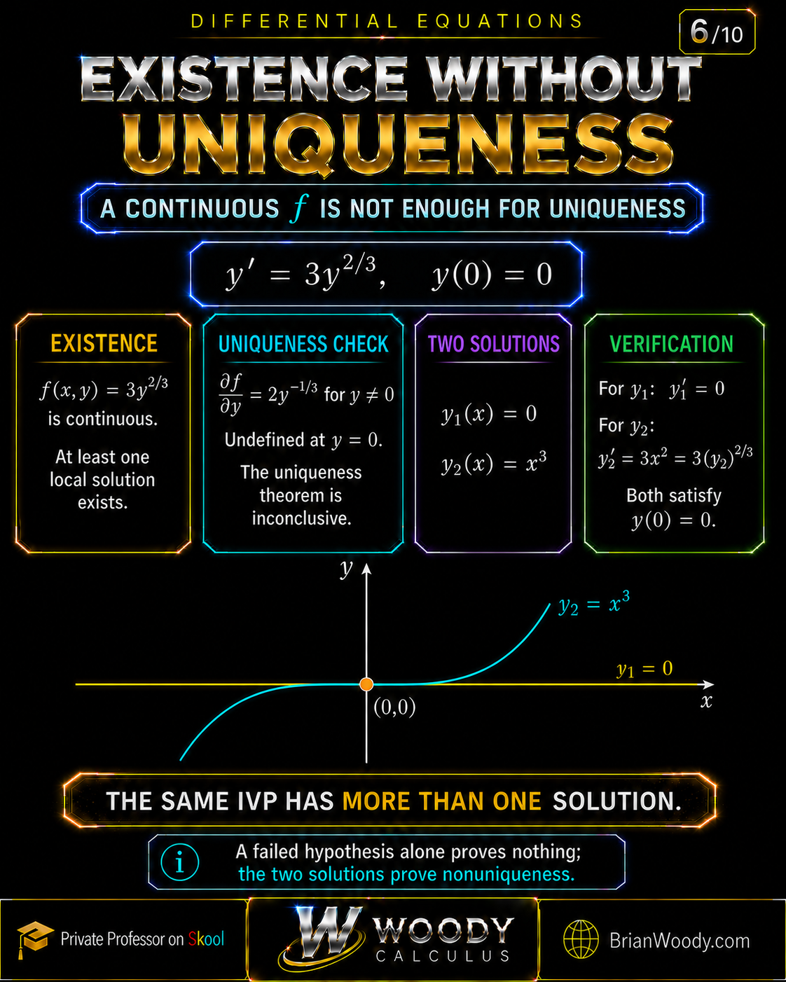
Existence Without Uniqueness: \(y^{\prime}=3y^{2/3}\), \(y(0)=0\)
Consider
The function \(f(x,y)=3y^{2/3}\) is continuous for every real \(y\), so at least one local solution exists. However,
and this derivative is undefined at \(y=0\). The standard uniqueness test is therefore inconclusive at the initial point.
Two solutions prove nonuniqueness
Solution 1
\(y_1(x)=0\)
Then \(y_1^{\prime}=0=3(0)^{2/3}\).
Solution 2
\(y_2(x)=x^3\)
Then \(y_2^{\prime}=3x^2\).
Using the real cube-root convention,
3\left(x^3\right)^{2/3}
=3\left(\sqrt[3]{x^3}\right)^2
=3x^2
=y_2^{\prime}.
\]
Both solutions satisfy \(y(0)=0\), so the IVP is not unique. Notice the logic: the failed derivative hypothesis proves nothing by itself; the two verified solutions prove nonuniqueness.
In fact, there are infinitely many solutions
For every waiting time \(a\ge 0\), define
y_a(x)=
\begin{cases}
0, & x\le a,\\
(x-a)^3, & x\ge a.
\end{cases}
\]
At \(x=a\), both pieces have value \(0\) and derivative \(0\), so \(y_a\) is differentiable and satisfies the ODE. Because \(a\ge0\), every member of this family also satisfies \(y_a(0)=0\). The solution may remain at equilibrium and then depart after any chosen waiting time.
When the ODE Is Undefined at the Initial Point
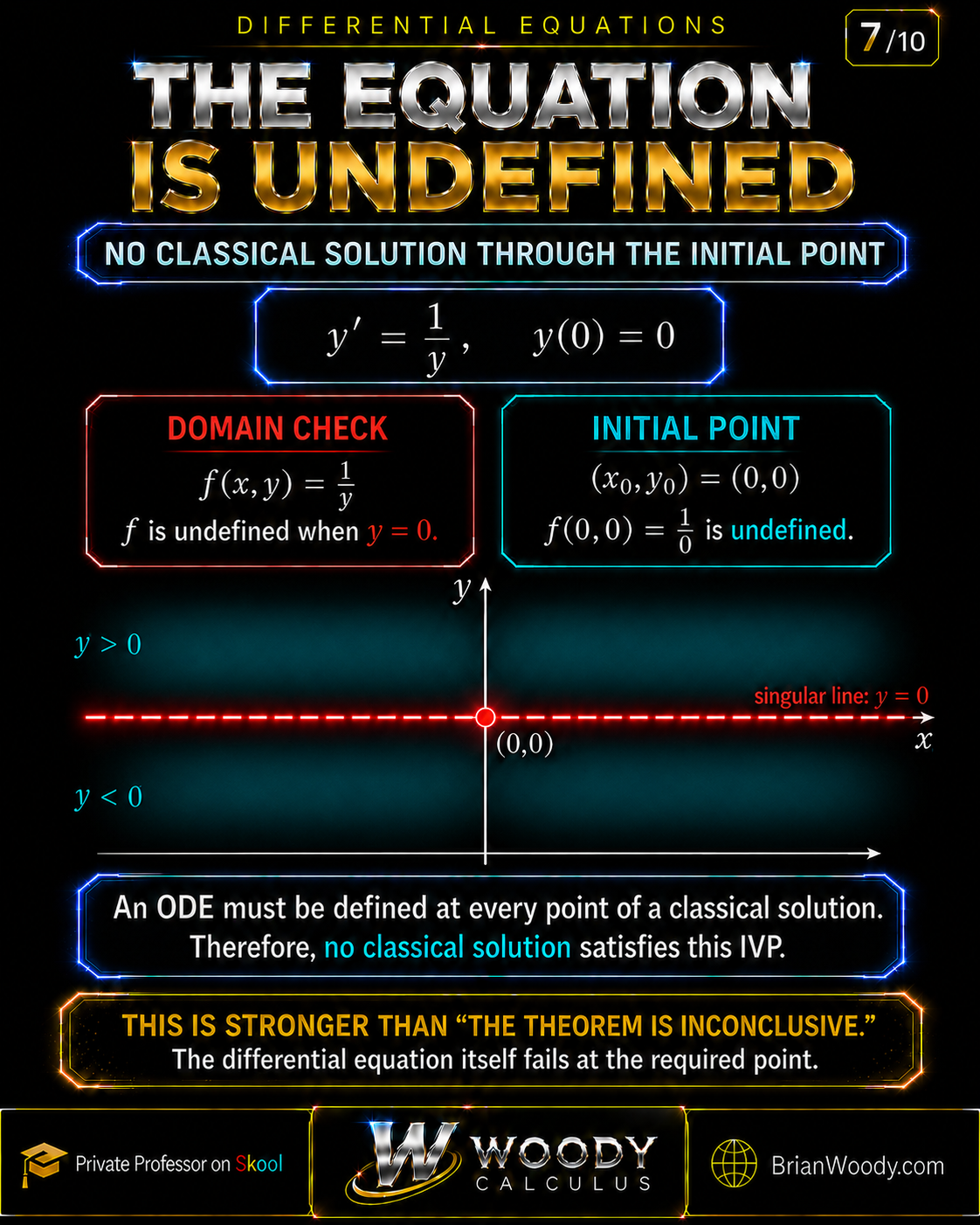
Consider
The right-hand side \(f(x,y)=1/y\) is undefined along the entire line \(y=0\). In particular, \(f(0,0)\) does not exist.
A classical solution must be differentiable and must satisfy \(y^{\prime}(x)=f(x,y(x))\) at every point of its interval, including the initial point. That requirement is impossible here. Therefore, no classical solution satisfies this IVP.
Why formal separation does not rescue the IVP
Away from \(y=0\), separation gives \(y\,dy=dx\), hence \(y^2=2x+C\). Formally inserting \((0,0)\) gives \(y=\pm\sqrt{2x}\), but these curves have an infinite derivative at \(x=0\), and \(1/y\) is still undefined there. They are not classical solutions of the stated IVP.
Local Existence Does Not Automatically Mean Global Existence
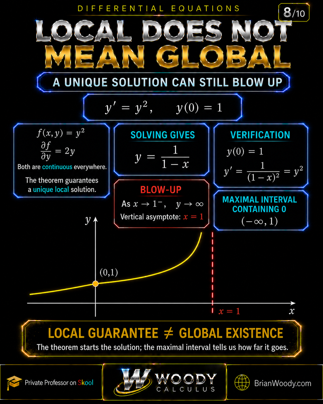
Consider the nonlinear IVP
Here \(f(x,y)=y^2\) and \(f_y(x,y)=2y\) are continuous everywhere. Thus the theorem guarantees a unique local solution.
Separate variables:
\frac{dy}{y^2}=dx
\quad\Longrightarrow\quad
-\frac1y=x+C.
\]
Using \(y(0)=1\) gives \(C=-1\), so
The verification is immediate:
y^{\prime}=\frac1{(1-x)^2}=y^2,
\qquad y(0)=1.
\]
But the solution becomes unbounded as \(x\to1^-\). Its maximal interval containing \(x_0=0\) is
This is finite-time blow-up. The differential equation is smooth everywhere, yet the particular solution cannot be continued through \(x=1\) as a finite classical solution.
Higher-Order Linear Existence and Uniqueness
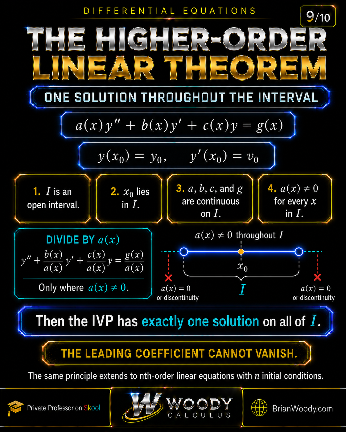
Linear equations receive a stronger interval-wide conclusion. Consider
a(x)y^{\prime\prime}+b(x)y^{\prime}+c(x)y=g(x),
\qquad y(x_0)=y_0,\quad y^{\prime}(x_0)=v_0.
\]
LINEAR THEOREM
Suppose \(a,b,c,g\) are continuous on an open interval \(I\), \(x_0\in I\), and \(a(x)\ne0\) for every \(x\in I\). Then the IVP has exactly one solution defined throughout \(I\).
The nonvanishing leading coefficient allows us to divide by \(a(x)\) and write the equation in standard form with continuous coefficients. The same principle extends to an \(n\)th-order linear equation when the normalized coefficients and forcing term are continuous on the interval.
Why Unique Solution Curves Cannot Intersect
Suppose \(y_1\) and \(y_2\) solve the same ODE inside a region where the uniqueness hypotheses hold. If their graphs meet at \((x_*,y_*)\), then both satisfy the same IVP
Uniqueness forces the two solutions to coincide wherever both are defined in the connected uniqueness region. Therefore, genuinely distinct solution curves cannot intersect there—not even tangentially.
This explains why the curves \(y=0\) and \(y=x^3\) may meet in the nonunique example: the uniqueness condition fails precisely at \(y=0\).
The Complete Existence and Uniqueness Decision Map

Six Common Existence and Uniqueness Mistakes
1. Treating existence and uniqueness as one claim
Continuity of \(f\) gives existence, not automatically uniqueness.
2. Saying “no solution” when a hypothesis fails
Failure of continuity usually means the theorem is inconclusive, not that no solution exists.
3. Saying “nonunique” because \(f_y\) is discontinuous
You still need two solutions or another proof of nonuniqueness.
4. Ignoring the initial point
A rectangle is useful only if it contains \((x_0,y_0)\) and avoids the relevant discontinuities.
5. Confusing local and global existence
A locally unique solution may encounter a singularity or blow up in finite time.
6. Forgetting to verify an explicit solution
Check both the differential equation and every initial condition.
Woody Mastery Check
Try each problem before opening the solution. The goal is to state only what the theorem actually guarantees.
1. What does the theorem say about \(y^{\prime}=x^2+y^2\), \(y(0)=0\)?
Here \(f(x,y)=x^2+y^2\) and \(f_y(x,y)=2y\) are continuous everywhere. Therefore, the IVP has exactly one local solution. The theorem alone does not guarantee that this nonlinear solution exists for every real \(x\).
2. What can the standard test conclude for \(y^{\prime}=\sqrt{|y|}\), \(y(0)=0\)?
The function \(f(y)=\sqrt{|y|}\) is continuous, so at least one local solution exists. Its derivative with respect to \(y\) is not continuous at \(0\), so the standard uniqueness test is inconclusive. Indeed, the IVP is nonunique, but that requires a separate demonstration.
3. Find the maximal interval for \(y^{\prime}=1/(x-2)\), \(y(0)=1\).
Integrating gives \(y=\ln|x-2|+C\). The initial condition yields \(C=1-\ln2\), so \(y=1+\ln(|x-2|/2)\). The interval containing \(0\) cannot cross \(x=2\), so the maximal interval is \((-\infty,2)\).
4. Why does \(a(x)\ne0\) matter in a second-order linear theorem?
It allows division by the leading coefficient so the equation can be written as \(y^{\prime\prime}+p(x)y^{\prime}+q(x)y=r(x)\) with continuous normalized coefficients. If \(a\) vanishes, the equation may become singular or lose differential order.
Existence and Uniqueness Glossary
Frequently Asked Questions
What is the existence and uniqueness theorem for differential equations?
For \(y^{\prime}=f(x,y)\), \(y(x_0)=y_0\), continuity of \(f\) near \((x_0,y_0)\) guarantees at least one local solution. If \(\partial f/\partial y\) is also continuous there, the local solution is unique.
What is the difference between existence and uniqueness?
Existence means at least one solution satisfies the IVP. Uniqueness means there is only one such local solution. A problem may have existence without uniqueness.
Does continuity of \(f\) guarantee uniqueness?
No. Continuity of \(f\) guarantees local existence under the theorem, but uniqueness requires an additional condition such as local Lipschitz continuity in \(y\). Continuity of \(\partial f/\partial y\) is a standard sufficient test.
What if \(\partial f/\partial y\) is not continuous?
The standard derivative-based uniqueness test is inconclusive. The IVP might still be unique, or it might have multiple solutions. A separate argument is required.
Can two solution curves cross?
Inside a uniqueness region, genuinely distinct solutions of the same ODE cannot intersect. If two solutions meet at one point, uniqueness forces them to coincide on their common connected interval.
Why does \(y^{\prime}=1/y\), \(y(0)=0\) have no classical solution?
The right-hand side \(1/y\) is undefined at the required initial point. A classical solution must satisfy the ODE at that point, so no classical solution can meet the stated IVP.
Does local uniqueness imply global existence?
No. The IVP \(y^{\prime}=y^2\), \(y(0)=1\) has a unique local solution \(y=1/(1-x)\), but it blows up at \(x=1\). Its maximal interval containing the initial point is \((-\infty,1)\).
What is a maximal interval of existence?
It is the largest connected interval containing \(x_0\) on which the particular classical solution exists. Its endpoints may be determined by singularities, domain restrictions, or solution blow-up.
What is the higher-order linear existence and uniqueness theorem?
If the coefficients and forcing term of a linear ODE are continuous on an open interval and the leading coefficient never vanishes there, prescribed initial values determine exactly one solution throughout that interval.
Is continuity of \(\partial f/\partial y\) necessary for uniqueness?
No. It is sufficient, not necessary. For example, \(f(y)=|y|\) is locally Lipschitz and gives uniqueness even though \(\partial f/\partial y\) is undefined at \(y=0\).
References and Further Reading
The theorem statements, terminology, and examples in this original Woody Calculus lesson are consistent with standard undergraduate differential-equations treatments, including:
- Dennis G. Zill, A First Course in Differential Equations with Modeling Applications.
- William E. Boyce, Richard C. DiPrima, and Douglas B. Meade, Elementary Differential Equations and Boundary Value Problems.
- Earl A. Coddington, An Introduction to Ordinary Differential Equations.