Parametric equations are one of the first places in Calculus 2 where a graph stops being just a static picture and becomes a moving object.
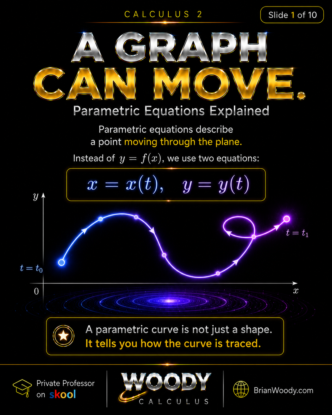
Instead of describing a curve with one equation such as \(y=f(x)\), parametric equations describe a point moving through the plane:
x=x(t),\qquad y=y(t).
\]
The parameter \(t\) controls the motion. For each value of \(t\), the equations produce one point \((x,y)\). As \(t\) changes, that point traces a path.
That is the key idea:
A parametric curve is not just a shape. It is a path with direction, speed, and motion.
This Woody Calculus lesson explains parametric equations in the way Calculus 2 students actually need them: how to generate points, trace direction, compute \(\frac{dx}{dt}\) and \(\frac{dy}{dt}\), find \(\frac{dy}{dx}\), identify horizontal tangents, identify vertical tangents, and avoid the common self-intersection trap.
Estimated read time: 15–20 minutes.
Last updated: .
What Are Parametric Equations?
Parametric equations describe a curve using a third variable, usually called \(t\). Instead of writing \(y\) directly as a function of \(x\), we describe both coordinates separately:
x=x(t),\qquad y=y(t).
\]
The variable \(t\) is called the parameter. You can think of \(t\) as time, although it does not always literally represent time. For every value of \(t\), the equations give one point:
t\longmapsto (x(t),y(t)).
\]
As \(t\) changes, the point moves. That movement is what makes parametric equations powerful.
A regular Cartesian equation usually tells you where a curve is. A parametric equation also tells you how the curve is traced.
The Parameter Controls the Point
Consider the parametric equations:
x=t^2-4,\qquad y=t^3-3t.
\]
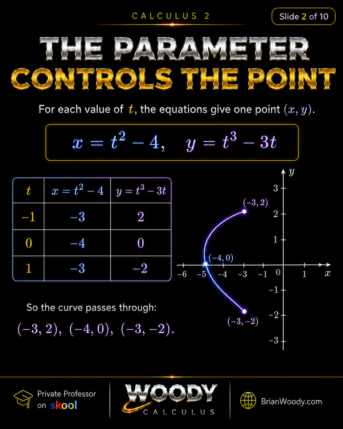
For each value of \(t\), we get one point \((x,y)\). Here are a few sample values:
| \(t\) | \(x=t^2-4\) | \(y=t^3-3t\) | Point \((x,y)\) |
|---|---|---|---|
| \(-2\) | \(0\) | \(-2\) | \((0,-2)\) |
| \(-1\) | \(-3\) | \(2\) | \((-3,2)\) |
| \(0\) | \(-4\) | \(0\) | \((-4,0)\) |
| \(1\) | \(-3\) | \(-2\) | \((-3,-2)\) |
| \(2\) | \(0\) | \(2\) | \((0,2)\) |
The parameter \(t\) is not just a calculator input. It controls the position of the moving point.
Parametric Curves Have Direction
One of the most important differences between Cartesian graphs and parametric curves is direction.
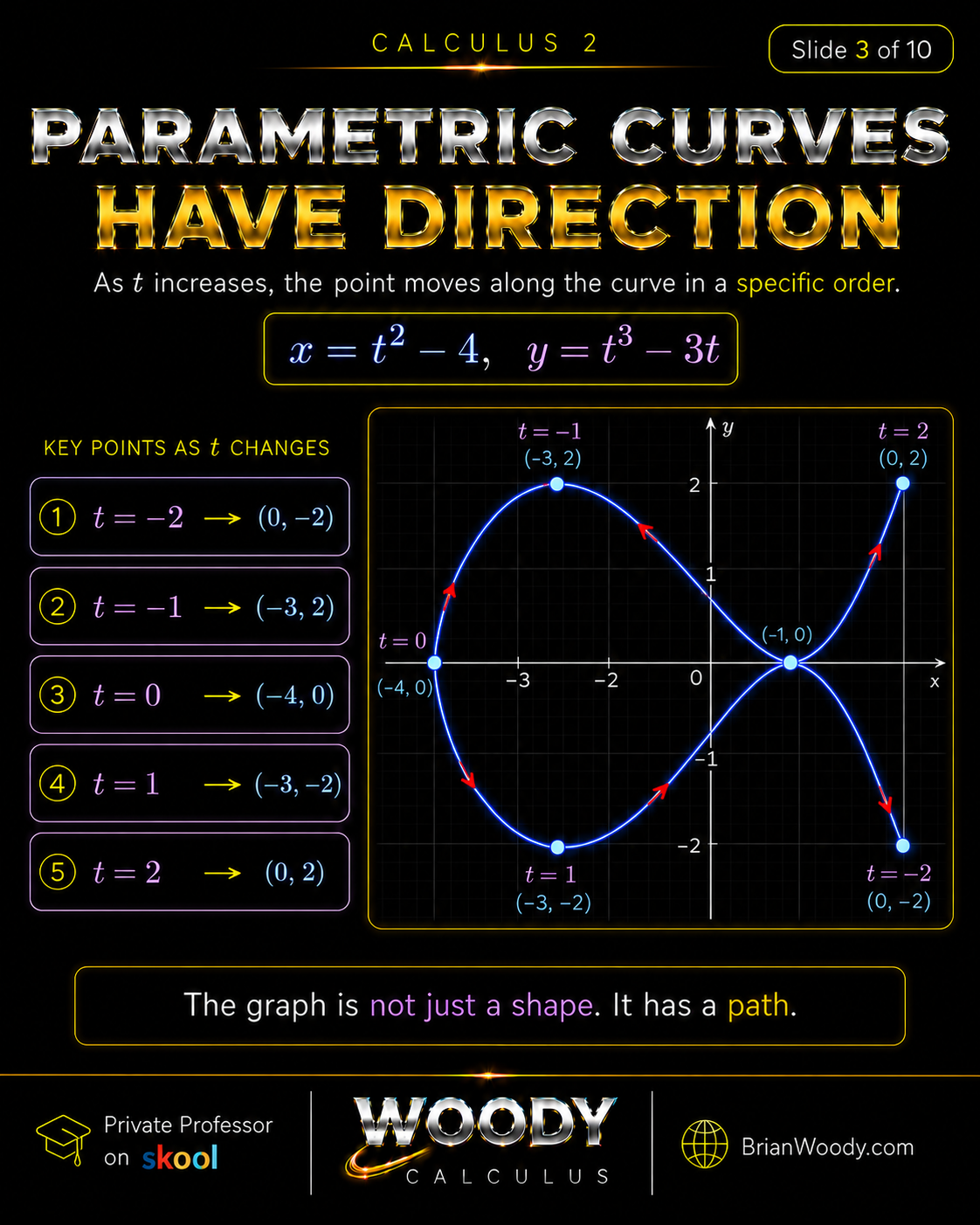
A Cartesian equation may describe the shape of a curve. A parametric equation describes how the point moves along the curve as \(t\) increases.
For the example:
x=t^2-4,\qquad y=t^3-3t,
\]
the point moves through the following ordered values:
t=-2\to (0,-2),
\qquad
t=-1\to (-3,2),
\qquad
t=0\to (-4,0),
\]
t=1\to (-3,-2),
\qquad
t=2\to (0,2).
\]
The curve is not merely a set of points. It is a path.
This matters in problems involving tangent lines, velocity, motion, arc length, and vector-valued curves.
Differentiate Each Coordinate
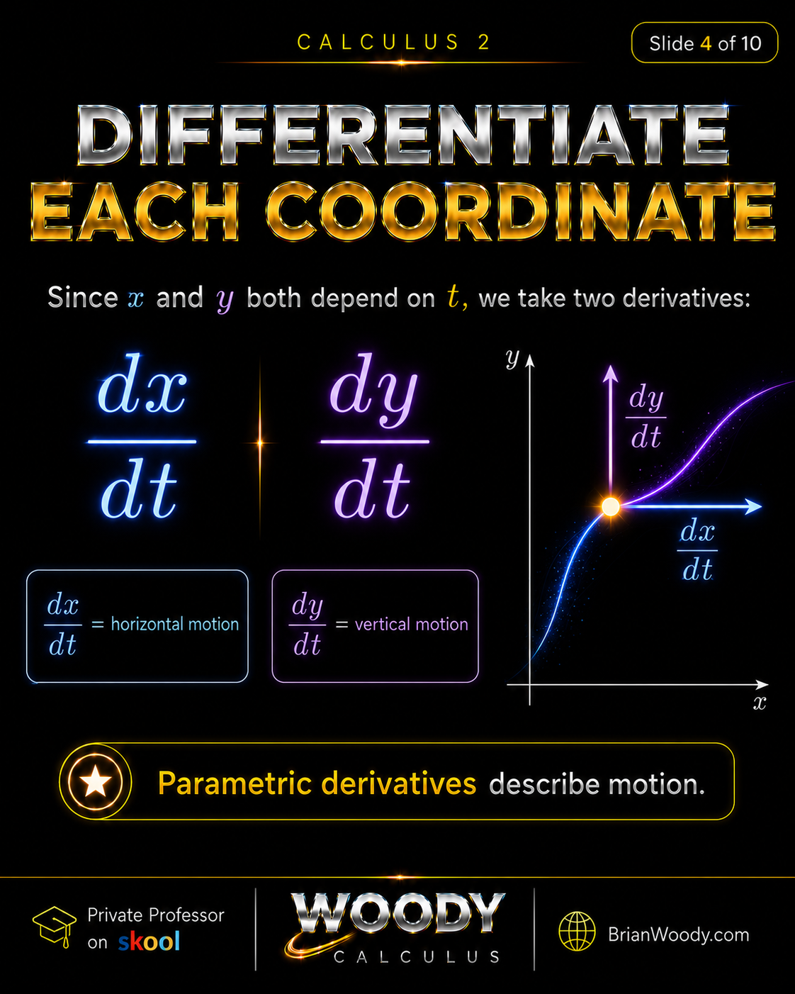
Since \(x\) and \(y\) both depend on \(t\), we differentiate each coordinate with respect to \(t\):
\frac{dx}{dt},\qquad \frac{dy}{dt}.
\]
These derivatives have a geometric meaning:
- \(\frac{dx}{dt}\) measures horizontal motion.
- \(\frac{dy}{dt}\) measures vertical motion.
If \(\frac{dx}{dt}>0\), the point is moving to the right. If \(\frac{dx}{dt}<0\), the point is moving to the left. If \(\frac{dx}{dt}=0\), the point has no horizontal motion at that instant.
If \(\frac{dy}{dt}>0\), the point is moving upward. If \(\frac{dy}{dt}<0\), the point is moving downward. If \(\frac{dy}{dt}=0\), the point has no vertical motion at that instant.
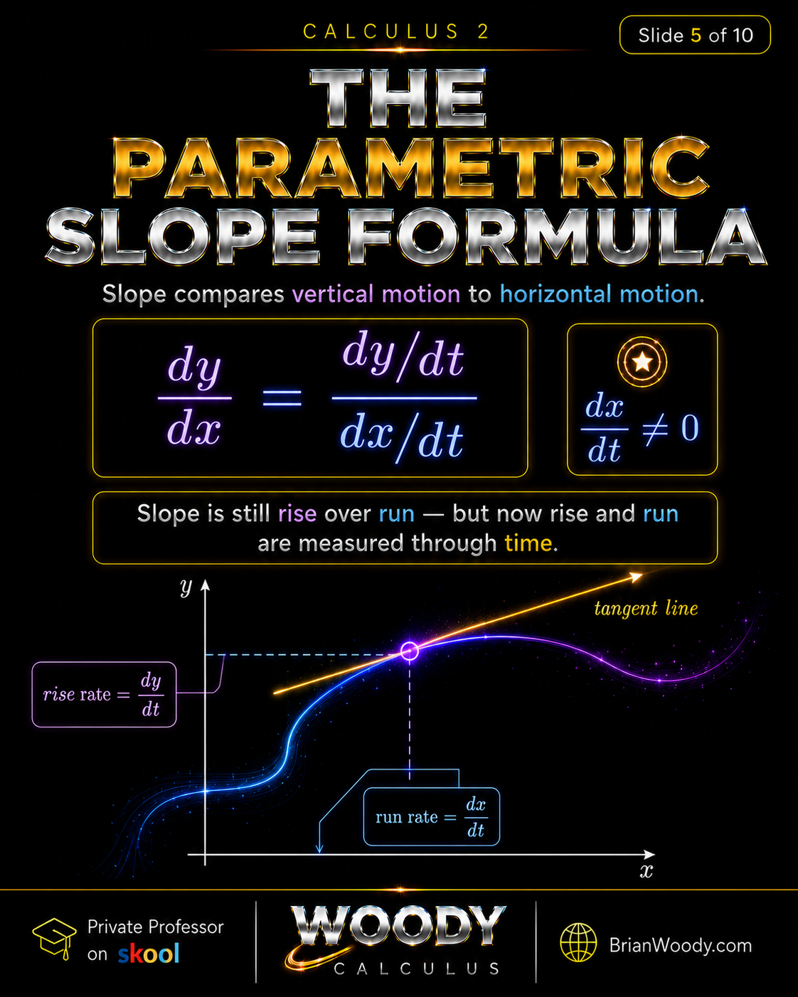
The Parametric Slope Formula
In ordinary Calculus, slope is:
\frac{dy}{dx}.
\]
For parametric equations, \(x\) and \(y\) both depend on \(t\). So slope compares vertical motion to horizontal motion:
\frac{dy}{dx}
=
\frac{\frac{dy}{dt}}{\frac{dx}{dt}},
\qquad
\frac{dx}{dt}\ne 0.
\]
This formula says:
Parametric slope equals vertical rate divided by horizontal rate.
It is still rise over run, but now both rise and run are measured through time.
How to Find Horizontal Tangents for Parametric Equations
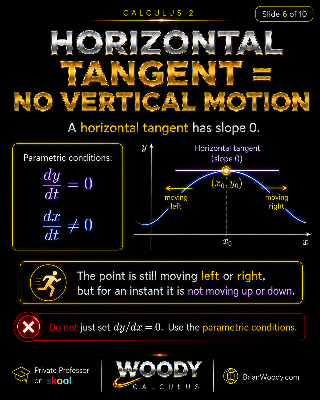
A horizontal tangent has slope \(0\). For parametric equations, that means vertical motion stops while horizontal motion continues.
The parametric conditions for a horizontal tangent are:
\frac{dy}{dt}=0,
\qquad
\frac{dx}{dt}\ne 0.
\]
The first condition makes the numerator of \(\frac{dy}{dx}\) equal to zero. The second condition prevents division by zero.
So the correct method is not simply “set \(\frac{dy}{dx}=0\).” The safer method is:
- Set \(\frac{dy}{dt}=0\).
- Solve for \(t\).
- Check that \(\frac{dx}{dt}\ne 0\).
- Plug valid \(t\)-values into \(x(t)\) and \(y(t)\).
How to Find Vertical Tangents for Parametric Equations
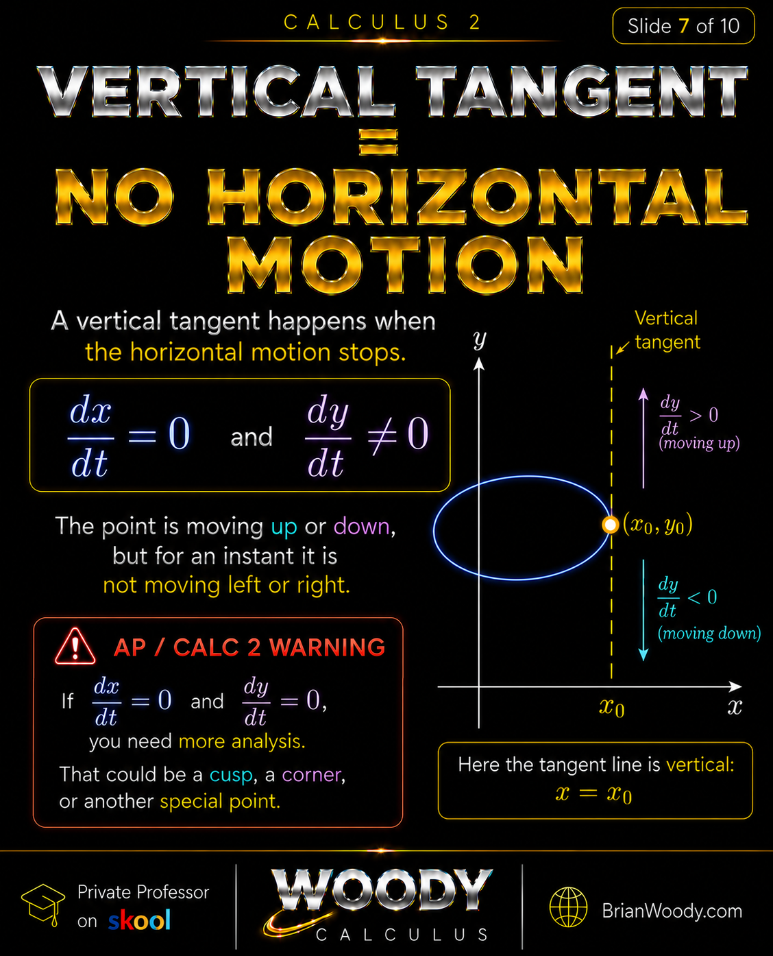
A vertical tangent happens when horizontal motion stops while vertical motion continues.
The parametric conditions for a vertical tangent are:
\frac{dx}{dt}=0,
\qquad
\frac{dy}{dt}\ne 0.
\]
This makes the denominator of the parametric slope formula zero while the numerator remains nonzero.
The correct method is:
- Set \(\frac{dx}{dt}=0\).
- Solve for \(t\).
- Check that \(\frac{dy}{dt}\ne 0\).
- Plug valid \(t\)-values into \(x(t)\) and \(y(t)\).
If both derivatives are zero:
\frac{dx}{dt}=0
\qquad\text{and}\qquad
\frac{dy}{dt}=0,
\]
then the point requires more analysis. It may be a cusp, a corner, a stationary point, or another special point. Do not automatically call it a horizontal or vertical tangent.
Example: Derivatives and Tangent Hunt
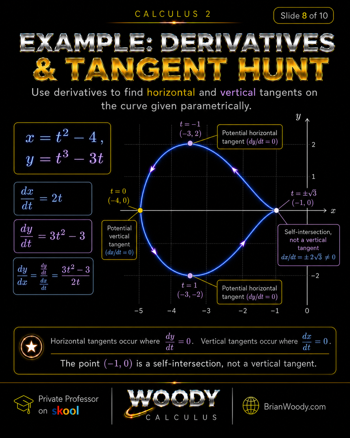
Now use the example:
x=t^2-4,\qquad y=t^3-3t.
\]
Differentiate each coordinate:
\frac{dx}{dt}=2t,
\qquad
\frac{dy}{dt}=3t^2-3.
\]
The parametric slope formula gives:
\frac{dy}{dx}
=
\frac{3t^2-3}{2t},
\qquad t\ne 0.
\]
This formula helps us search for horizontal and vertical tangents, but the safest method is still to analyze \(\frac{dx}{dt}\) and \(\frac{dy}{dt}\) separately.
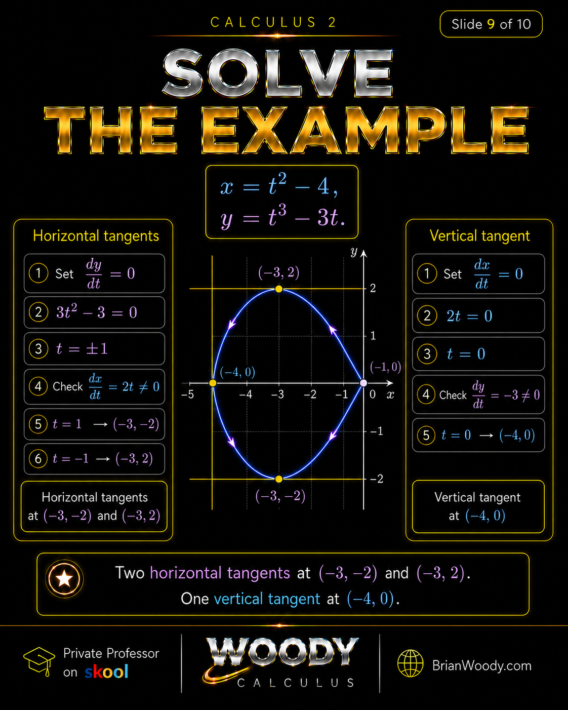
Solve the Example
Horizontal Tangents
Horizontal tangents occur where:
\frac{dy}{dt}=0,
\qquad
\frac{dx}{dt}\ne 0.
\]
Set:
3t^2-3=0.
\]
Then:
3(t^2-1)=0
\quad\Longrightarrow\quad
t^2=1
\quad\Longrightarrow\quad
t=\pm 1.
\]
Check \(\frac{dx}{dt}=2t\):
t=-1\Rightarrow \frac{dx}{dt}=-2\ne 0,
\qquad
t=1\Rightarrow \frac{dx}{dt}=2\ne 0.
\]
So both values give horizontal tangents.
Find the points:
t=-1:
\quad
x=(-1)^2-4=-3,
\qquad
y=(-1)^3-3(-1)=2.
\]
t=1:
\quad
x=1^2-4=-3,
\qquad
y=1^3-3(1)=-2.
\]
Therefore, the horizontal tangent points are:
\boxed{(-3,2)\quad\text{and}\quad (-3,-2).}
\]
The corresponding horizontal tangent lines are:
\boxed{y=2\quad\text{and}\quad y=-2.}
\]
Vertical Tangent
Vertical tangents occur where:
\frac{dx}{dt}=0,
\qquad
\frac{dy}{dt}\ne 0.
\]
Set:
2t=0.
\]
Then:
t=0.
\]
Check \(\frac{dy}{dt}\):
\frac{dy}{dt}=3(0)^2-3=-3\ne 0.
\]
So \(t=0\) gives a vertical tangent.
Find the point:
x=0^2-4=-4,
\qquad
y=0^3-3(0)=0.
\]
Therefore, the vertical tangent point is:
\boxed{(-4,0).}
\]
The corresponding vertical tangent line is:
\boxed{x=-4.}
\]
How to Find Self-Intersections on Parametric Curves
The point \((-1,0)\) is a self-intersection on this curve, but it is not a vertical tangent.
To see why, solve:
x=t^2-4=-1.
\]
Then:
t^2=3
\quad\Longrightarrow\quad
t=\pm\sqrt{3}.
\]
At both values:
y=t^3-3t=t(t^2-3)=0.
\]
So both \(t=\sqrt{3}\) and \(t=-\sqrt{3}\) give the point \((-1,0)\).
But the horizontal derivative is:
\frac{dx}{dt}=2t.
\]
At \(t=\pm\sqrt{3}\):
\frac{dx}{dt}=\pm 2\sqrt{3}\ne 0.
\]
So the point \((-1,0)\) is not a vertical tangent. It is a self-intersection with two different parameter values.
The slopes at the self-intersection are:
\frac{dy}{dx}
=
\frac{3t^2-3}{2t}.
\]
Since \(t^2=3\), we get:
\frac{dy}{dx}
=
\frac{6}{2t}
=
\frac{3}{t}.
\]
Thus:
t=\sqrt{3}\Rightarrow \frac{dy}{dx}=\sqrt{3},
\qquad
t=-\sqrt{3}\Rightarrow \frac{dy}{dx}=-\sqrt{3}.
\]
At the same point \((-1,0)\), the curve has two tangent directions:
\boxed{y=\sqrt{3}(x+1)}
\qquad
\text{and}
\qquad
\boxed{y=-\sqrt{3}(x+1)}.
\]
This is why parametric equations must be analyzed using \(t\), not just the visible point on the graph.
Complete Worked Example
Find the horizontal and vertical tangents for:
x=t^2-4,
\qquad
y=t^3-3t.
\]
First compute derivatives:
\frac{dx}{dt}=2t,
\qquad
\frac{dy}{dt}=3t^2-3.
\]
For horizontal tangents:
3t^2-3=0
\quad\Longrightarrow\quad
t=\pm 1.
\]
Both values have \(\frac{dx}{dt}\ne 0\), so both are valid. Plugging into \(x(t)\) and \(y(t)\), we get:
t=-1\Rightarrow (-3,2),
\qquad
t=1\Rightarrow (-3,-2).
\]
So the horizontal tangent lines are:
\boxed{y=2}
\qquad
\text{and}
\qquad
\boxed{y=-2}.
\]
For vertical tangents:
2t=0
\quad\Longrightarrow\quad
t=0.
\]
Since \(\frac{dy}{dt}=-3\ne 0\), this gives a vertical tangent. Plugging into the curve:
t=0\Rightarrow (-4,0).
\]
So the vertical tangent line is:
\boxed{x=-4}.
\]
Final answer:
\boxed{\text{Horizontal tangents: } y=2,\ y=-2.}
\]
\boxed{\text{Vertical tangent: } x=-4.}
\]
Plain-language answer: the curve has horizontal tangents at \((-3,2)\) and \((-3,-2)\), and one vertical tangent at \((-4,0)\).
Common Mistakes
Mistake 1: Treating the graph as only a shape
A parametric curve has direction. The same geometric curve can be traced in different ways depending on the parameterization.
Mistake 2: Forgetting to check the other derivative
For horizontal tangents, do not only solve \(\frac{dy}{dt}=0\). You must also check \(\frac{dx}{dt}\ne 0\).
For vertical tangents, do not only solve \(\frac{dx}{dt}=0\). You must also check \(\frac{dy}{dt}\ne 0\).
Mistake 3: Calling a self-intersection a vertical tangent
A self-intersection happens when two different \(t\)-values produce the same point. That does not automatically mean the tangent is vertical.
Mistake 4: Ignoring special points where both derivatives vanish
If:
\frac{dx}{dt}=0
\quad\text{and}\quad
\frac{dy}{dt}=0,
\]
then more analysis is needed. The point could be a cusp, corner, or another special point.
Mistake 5: Forgetting to plug \(t\) back into both equations
Solving for \(t\) is not the final answer. After finding \(t\), plug it into both \(x(t)\) and \(y(t)\) to get the point.
Parametric Equations Cheat Sheet
| Question | Condition | What to Check |
|---|---|---|
| Slope | \(\frac{dy}{dx}=\frac{dy/dt}{dx/dt}\) | \(\frac{dx}{dt}\ne 0\) |
| Horizontal tangent | \(\frac{dy}{dt}=0\) | \(\frac{dx}{dt}\ne 0\) |
| Vertical tangent | \(\frac{dx}{dt}=0\) | \(\frac{dy}{dt}\ne 0\) |
| Special point | \(\frac{dx}{dt}=0\) and \(\frac{dy}{dt}=0\) | More analysis required |
| Self-intersection | Two different \(t\)-values give the same \((x,y)\) | Analyze each \(t\)-value separately |
Parametric Equations FAQ
What are parametric equations?
Parametric equations describe a curve using a parameter, usually \(t\), with two equations \(x=x(t)\) and \(y=y(t)\). Each value of \(t\) gives one point on the curve.
Why do parametric curves have direction?
Parametric curves have direction because the point moves along the curve as \(t\) increases. The ordered values of \(t\) determine how the curve is traced.
How do you find \(\frac{dy}{dx}\) for parametric equations?
Use the formula \(\frac{dy}{dx}=\frac{dy/dt}{dx/dt}\), provided \(\frac{dx}{dt}\ne 0\). This compares vertical motion to horizontal motion.
When does a parametric curve have a horizontal tangent?
A parametric curve has a horizontal tangent when \(\frac{dy}{dt}=0\) and \(\frac{dx}{dt}\ne 0\).
When does a parametric curve have a vertical tangent?
A parametric curve has a vertical tangent when \(\frac{dx}{dt}=0\) and \(\frac{dy}{dt}\ne 0\).
What if both \(\frac{dx}{dt}\) and \(\frac{dy}{dt}\) are zero?
If both derivatives are zero, the point requires more analysis. It may be a cusp, a corner, a stationary point, or another special point.
How do you find horizontal and vertical tangents for \(x=t^2-4\), \(y=t^3-3t\)?
Compute \(\frac{dx}{dt}=2t\) and \(\frac{dy}{dt}=3t^2-3\). Horizontal tangents occur at \(t=\pm1\), giving \((-3,2)\) and \((-3,-2)\). The vertical tangent occurs at \(t=0\), giving \((-4,0)\).
Why is \((-1,0)\) a self-intersection and not a vertical tangent?
The point \((-1,0)\) occurs at \(t=\pm\sqrt{3}\). At those parameter values, \(\frac{dx}{dt}\ne 0\), so the point is not a vertical tangent. It is a self-intersection with two different tangent directions.
Master Parametric Equations with Woody Calculus
Parametric equations are not just a new graphing trick. They are a new way to think about motion, direction, velocity, slope, and tangent lines.
The Woody Calculus Method
The Woody Calculus method is built around strict formula memorization, visual structure, repeated perfect solutions, and saying each step out loud until the process becomes automatic.
- Understand that \(t\) controls the moving point.
- Make a table of values to see the curve.
- Track the order of the points as \(t\) increases.
- Differentiate \(x(t)\) and \(y(t)\) separately.
- Use \(\frac{dy}{dx}=\frac{dy/dt}{dx/dt}\) for slope.
- Use \(\frac{dy}{dt}=0\), \(\frac{dx}{dt}\ne 0\) for horizontal tangents.
- Use \(\frac{dx}{dt}=0\), \(\frac{dy}{dt}\ne 0\) for vertical tangents.
- Check self-intersections and special points carefully.
- Rewrite perfect solutions and say every step out loud until the method becomes automatic.
For students who want structured Calculus 2 help, join the Woody Calculus Mastery Lab. The Mastery Lab helps students build skill through repetition, step-by-step lessons, written solutions, exam-focused systems, and direct support.
You can also visit Woody Calculus on Skool for the learning community.
Related Woody Calculus Mathematical Essays
Explore more Woody Calculus lessons connecting Calculus 2, AP Calculus BC, parametric equations, tangent lines, arc length, improper integrals, integration techniques, infinite series, Taylor series, Differential Equations, and advanced mathematics.
- How to Learn Calculus and Advanced Mathematics: A Peak Performance Study Guide
- Trig Substitution Explained: The Woody Calculus 3-Type System
- Improper Integrals Explained: Calculus 2 Limit Problems
- Taylor Series Explained: Mathematical Time Travel in Calculus 2
- Radius of Convergence and Interval of Convergence Explained
- Gabriel’s Horn Explained: Finite Volume and Infinite Surface Area
- Laplace Transforms Explained: Differential Equations Become Algebra
- Line Integrals Explained: Vector Fields and Calculus 3
- View All Woody Calculus Blog Posts
Private Instruction
Brian M. Woody works privately with a limited number of serious students who need one-on-one help in AP Calculus BC, Calculus II, Calculus III, Differential Equations, and advanced mathematics.
Private instruction is reserved for serious students, requires weekly sessions, requires enrollment in the Woody Calculus Mastery Lab first, and approval is not guaranteed.
Students interested in private instruction can learn more here: Private Math Tutor and Advanced Mathematics Instruction.
Related University Math Help Pages
Woody Calculus supports students at major universities with structured help in Calculus 2, Calculus 3, Differential Equations, Linear Algebra, and advanced mathematics. For the full list of supported schools, visit the University Calculus Tutor Hub.
- University Calculus Tutor Hub
- AP Calculus BC Tutor
- Purdue University Calculus Tutor
- University of Florida Calculus Tutor
- Colorado State University Calculus Help
- UCF Calculus Tutor
- University of Nevada, Reno Calculus Tutor
- Auburn Calculus Tutor
- University of Alabama Calculus Tutor
- University of Wisconsin Calculus Tutor
- University of Michigan Calculus Tutor
- UCLA Calculus Tutor
- MIT Calculus Tutor
Trusted by Students Nationwide
The Woody Calculus Mastery Lab gives university students access to structured mathematics support, written solutions, video lessons, exam-focused training, and expert guidance from Brian M. Woody.
Students use Woody Calculus for Calculus II, Calculus III, Differential Equations, Linear Algebra, Abstract Algebra, and other advanced mathematics courses.