Original Woody Calculus Lesson
DIFFERENTIAL EQUATIONS · FIRST-ORDER ODEs · MODELING
How Do You Solve Mixing Problems in Differential Equations?
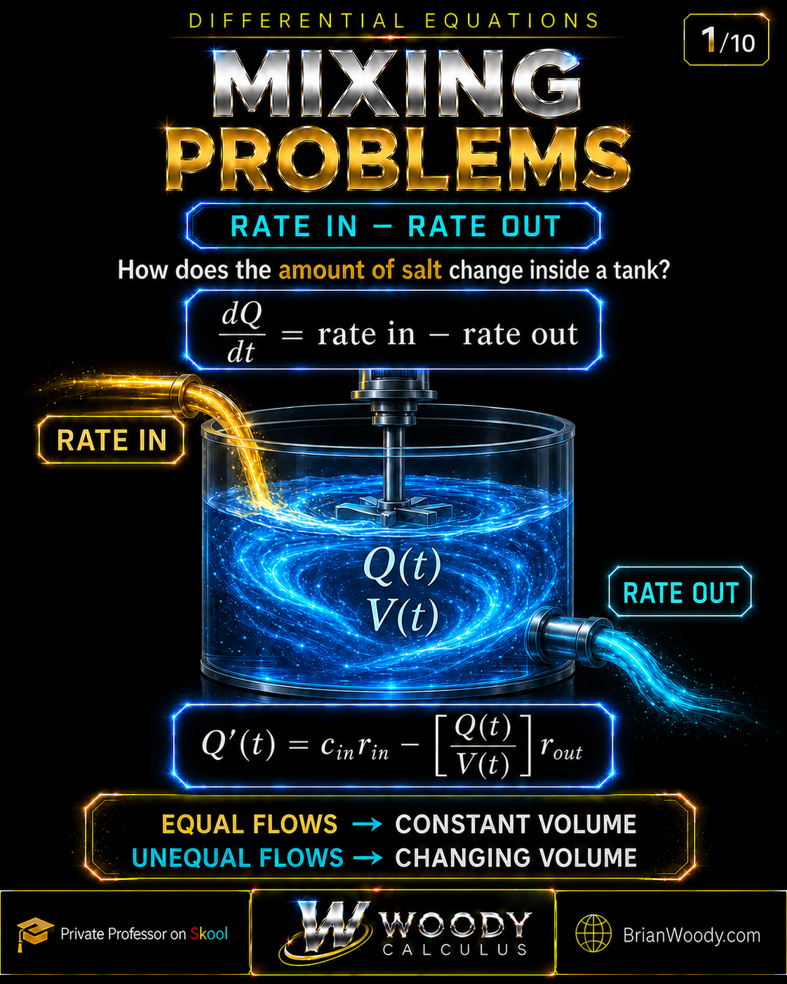
To solve a mixing problem, define the amount of dissolved substance, compute the tank volume, calculate the incoming and outgoing substance rates, and use the balance law “amount rate equals rate in minus rate out.” Perfect mixing makes the outgoing concentration equal to the current amount divided by the current volume. The result is usually a first-order linear initial-value problem.
Let \(Q(t)\) be the amount of salt and \(V(t)\) the solution volume. For constant volumetric flow rates,
The derivative of the amount of salt equals incoming concentration times incoming flow rate minus current tank concentration times outgoing flow rate.
\boxed{Q^{\prime}(t)=c_{\mathrm{in}}r_{\mathrm{in}}
-\frac{Q(t)}{V(t)}r_{\mathrm{out}}}
\]
Direct answer: Find the volume first, use the current tank concentration for the rate leaving, build the linear differential equation, solve the initial-value problem, and stop or change the model when the tank empties or reaches capacity.
Quick Summary
- Equal flows: the volume is constant and the linear ODE has a constant coefficient.
- Unequal flows: the volume changes and the rate-out coefficient usually depends on time.
- Physical interval: stop at the first emptying or overflow time unless the model is explicitly changed.
Estimated reading time: 40–50 minutes.
The Rate-In Minus Rate-Out Mixing Model
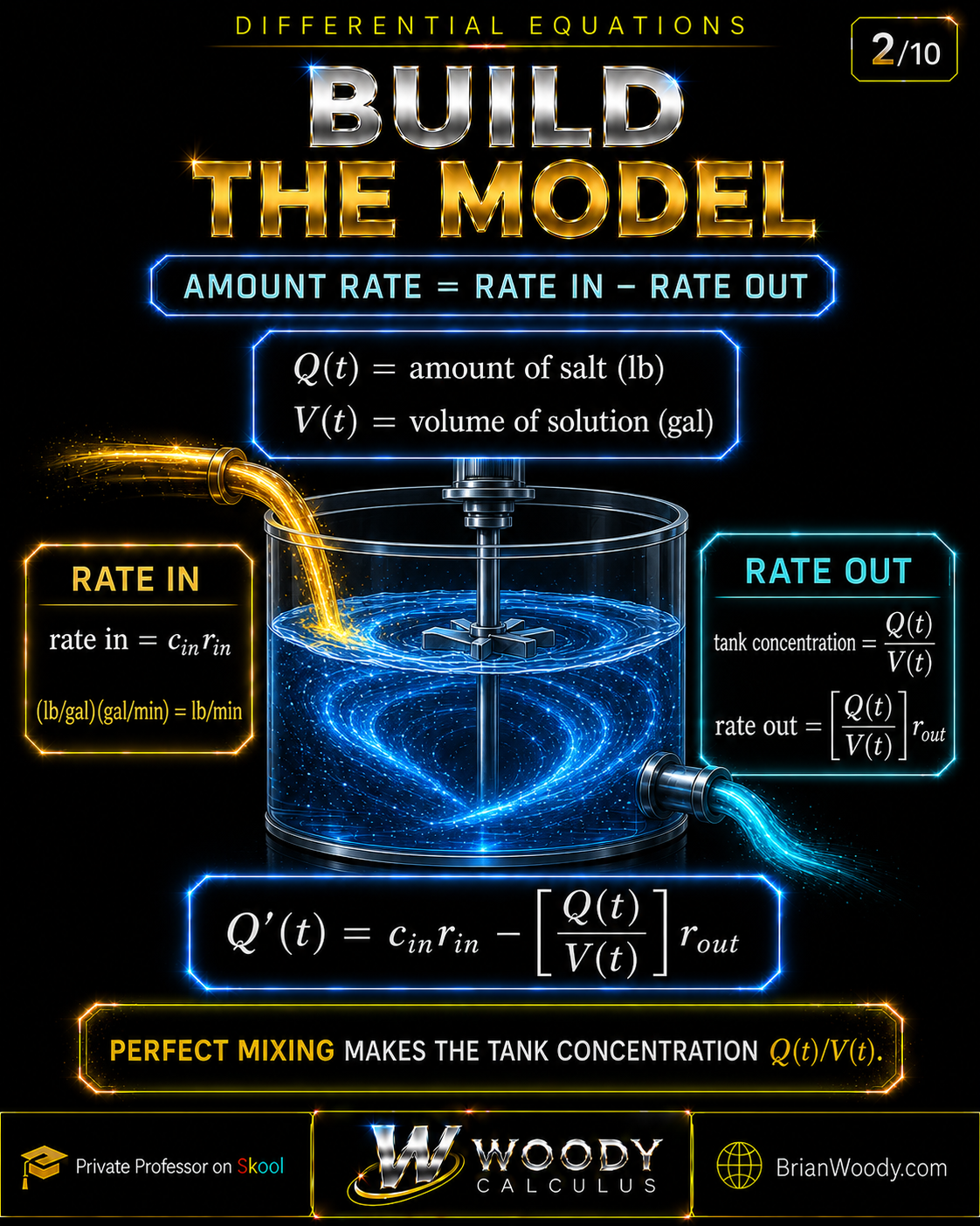
A mixing problem is a conservation or mass-balance model. The unknown is not usually the concentration itself. It is the amount of dissolved substance inside the tank.
Amount
\(Q(t)\) is the amount of salt or another dissolved substance, commonly measured in pounds, grams, or kilograms.
Volume
\(V(t)\) is the volume of liquid in the tank, commonly measured in gallons or liters.
Incoming rate
Incoming concentration multiplied by incoming volumetric flow gives substance per unit time.
Outgoing rate
Under perfect mixing, the outgoing concentration equals the current tank concentration \(Q(t)/V(t)\).
\text{rate in}=c_{\mathrm{in}}r_{\mathrm{in}},
\qquad
\text{rate out}=\frac{Q(t)}{V(t)}r_{\mathrm{out}}.
\]
| Quantity | Typical units | Meaning |
|---|---|---|
| \(Q(t)\) | lb | Amount of salt in the tank |
| \(V(t)\) | gal | Volume of solution |
| \(c_{\mathrm{in}}\) | lb/gal | Incoming concentration |
| \(r_{\mathrm{in}},r_{\mathrm{out}}\) | gal/min | Volumetric flow rates |
| \(Q^{\prime}(t)\) | lb/min | Net change in the amount of salt |
Why perfect mixing matters
The rate-out formula assumes that the concentration is uniform throughout the tank at each time. Without that assumption, one scalar function \(Q(t)\) is generally not enough to describe the spatial concentration.
How to Solve a Mixing Problem in Seven Steps
Use the same order every time. Most mistakes happen when students write the differential equation before determining the volume and the valid physical interval.
- 1
Define the amount and initial value
Let \(Q(t)\) be the amount of dissolved substance and translate the initial data into \(Q(0)=Q_0\).
- 2
Compute the volume and physical interval
For constant flow rates, use \(V(t)=V_0+(r_{\mathrm{in}}-r_{\mathrm{out}})t\), then find any emptying or overflow time.
- 3
Compute the incoming substance rate
Multiply incoming concentration by incoming volumetric flow: \(c_{\mathrm{in}}r_{\mathrm{in}}\).
- 4
Compute the outgoing substance rate
Use the current tank concentration: \([Q(t)/V(t)]r_{\mathrm{out}}\).
- 5
Write the initial-value problem
Apply \(Q^{\prime}=\text{rate in}-\text{rate out}\) and attach the initial condition.
- 6
Solve the linear differential equation
Put the ODE in standard linear form and use the integrating factor \(\mu(t)=e^{\int P(t)\,dt}\).
- 7
Verify the mathematics and the model
Check the ODE, initial condition, units, nonnegative quantities, and the physical time interval.
Variable flow-rate version
When the volumetric flow rates depend on time, replace the linear volume formula by
V(t)=V_0+\int_0^t\bigl(r_{\mathrm{in}}(s)-r_{\mathrm{out}}(s)\bigr)\,ds.
\]
Example 1: Equal Flow Rates and Constant Volume
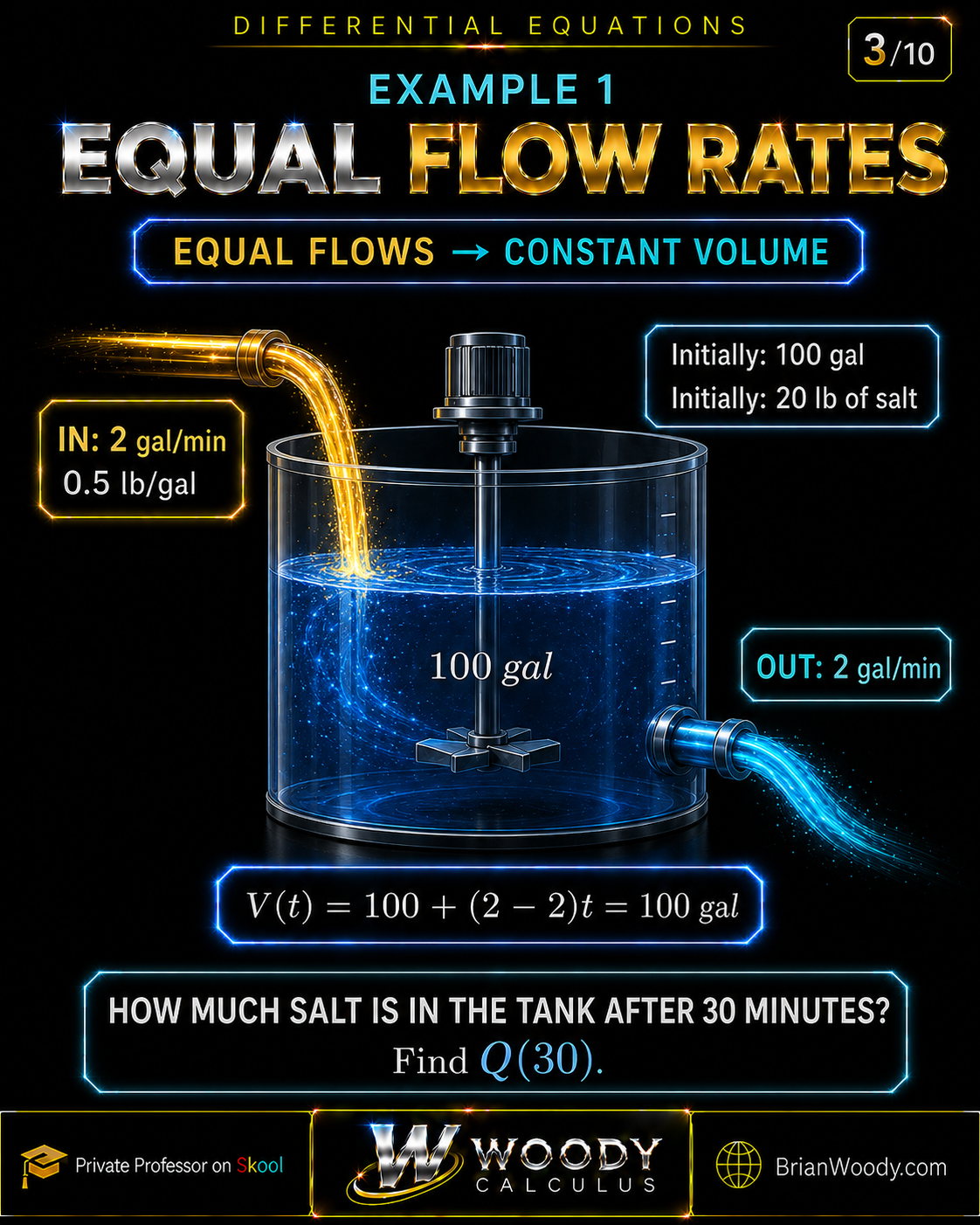
A tank initially contains 100 gallons of solution and 20 pounds of salt. Brine containing 0.5 pound of salt per gallon enters at 2 gallons per minute. The well-mixed solution leaves at 2 gallons per minute. Find the amount of salt after 30 minutes.
Step 1: Determine the volume
V(t)=100+(2-2)t=100\text{ gal}.
\]
Step 2: Build the rate equation
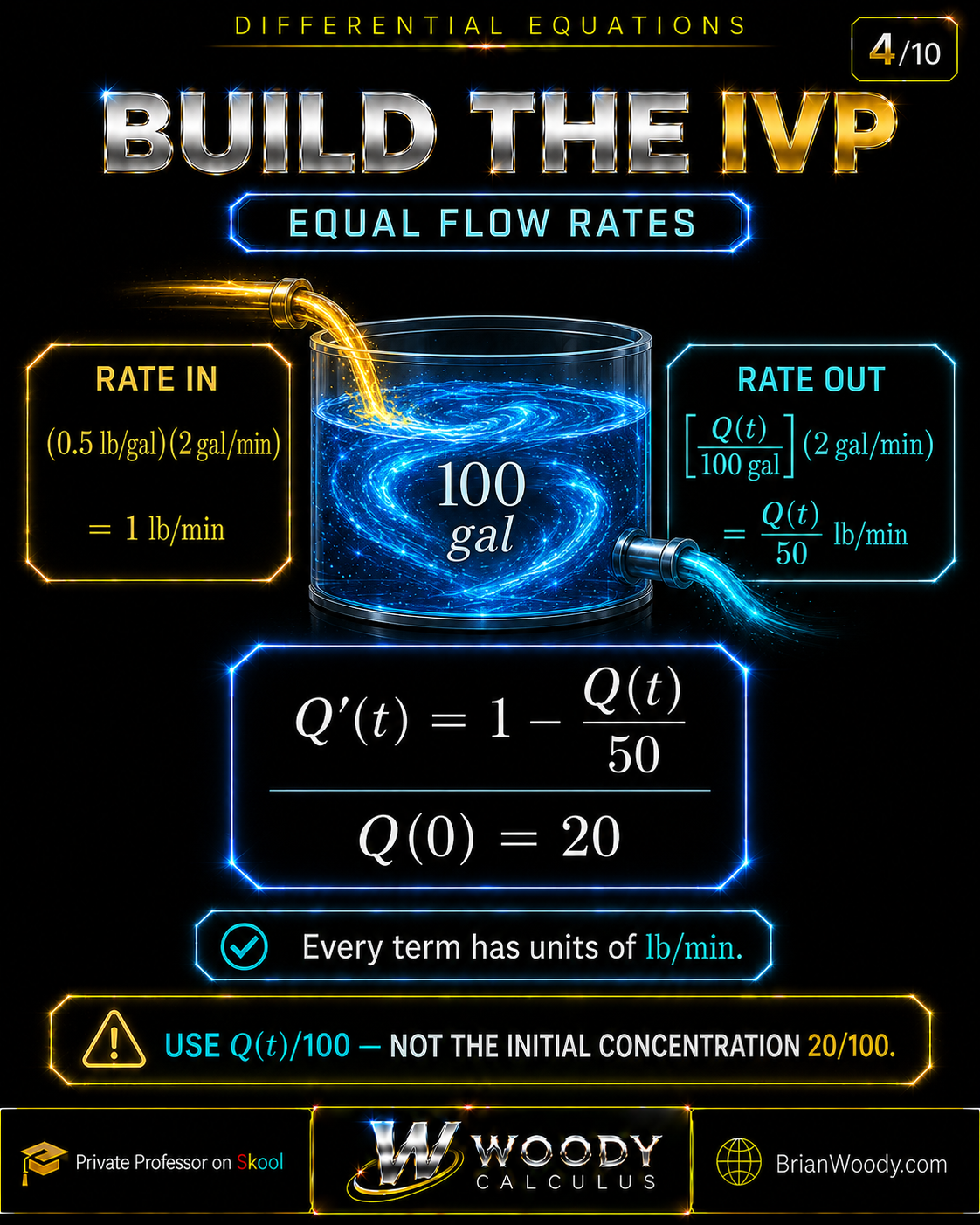
\text{rate in}=(0.5)(2)=1\text{ lb/min},
\]
\[
\text{rate out}=\frac{Q(t)}{100}(2)=\frac{Q(t)}{50}\text{ lb/min}.
\]
\boxed{Q^{\prime}=1-\frac{Q}{50},\qquad Q(0)=20.}
\]
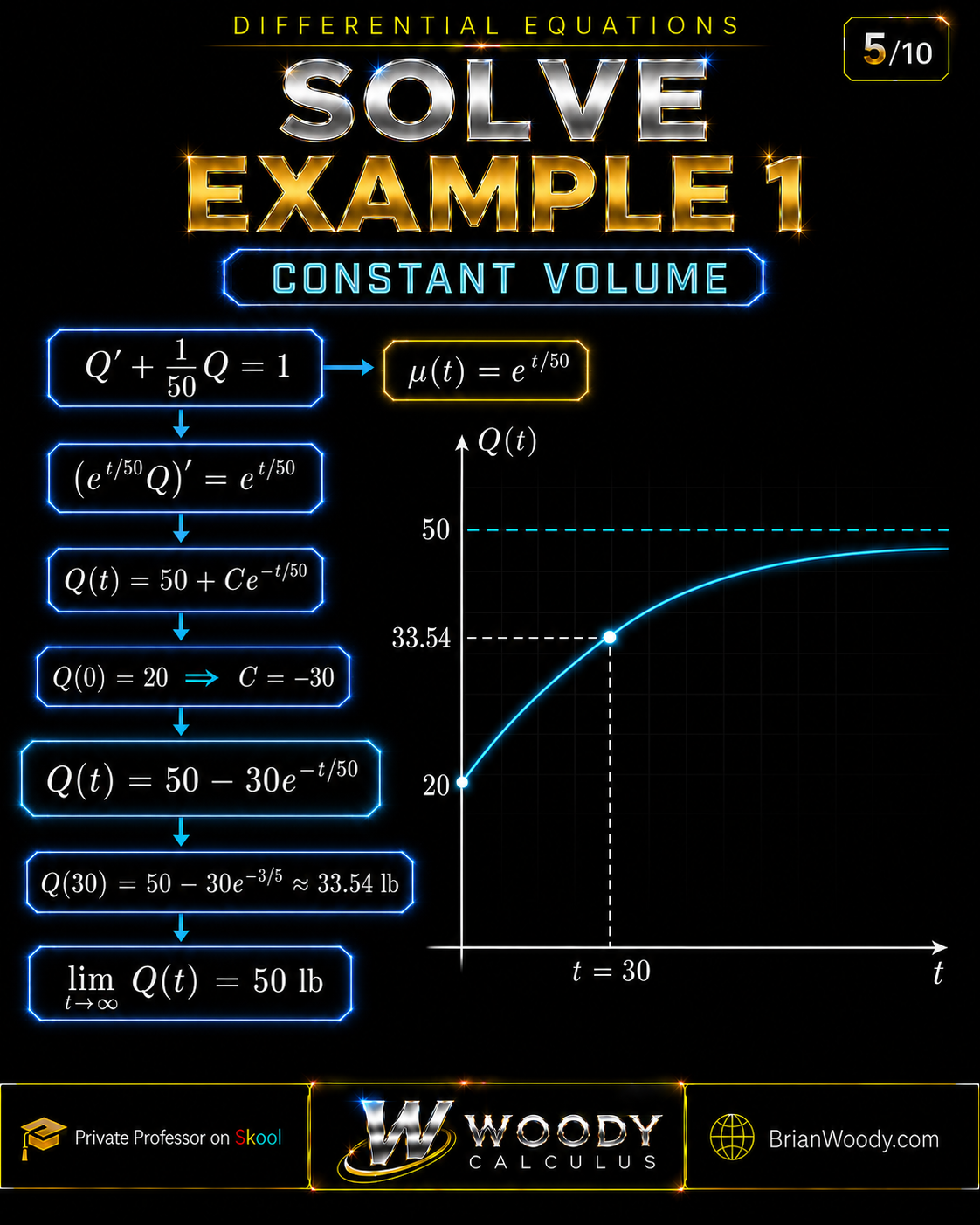
Step 3: Solve the linear IVP
Write the equation in standard form:
Q^{\prime}+\frac1{50}Q=1.
\]
The integrating factor is
\mu(t)=e^{\int(1/50)\,dt}=e^{t/50}.
\]
Therefore,
\bigl(e^{t/50}Q\bigr)^{\prime}=e^{t/50},
\]
\[
Q(t)=50+Ce^{-t/50}.
\]
Using \(Q(0)=20\) gives \(C=-30\). Hence
\boxed{Q(t)=50-30e^{-t/50}}.
\]
Q(30)=50-30e^{-3/5}\approx33.54\text{ lb}.
\]
Equilibrium, time constant, and physical meaning
Setting \(Q^{\prime}=0\) gives the equilibrium amount \(Q_{\mathrm{eq}}=50\) pounds. This agrees with the physical calculation \((0.5\text{ lb/gal})(100\text{ gal})=50\text{ lb}\). Moreover,
Q(t)-50=-30e^{-t/50}.
\]
The time constant is 50 minutes, and the remaining distance from equilibrium is halved every
50\ln2\approx34.66\text{ min}.
\]
Example 2: Unequal Flow Rates and a Draining Tank
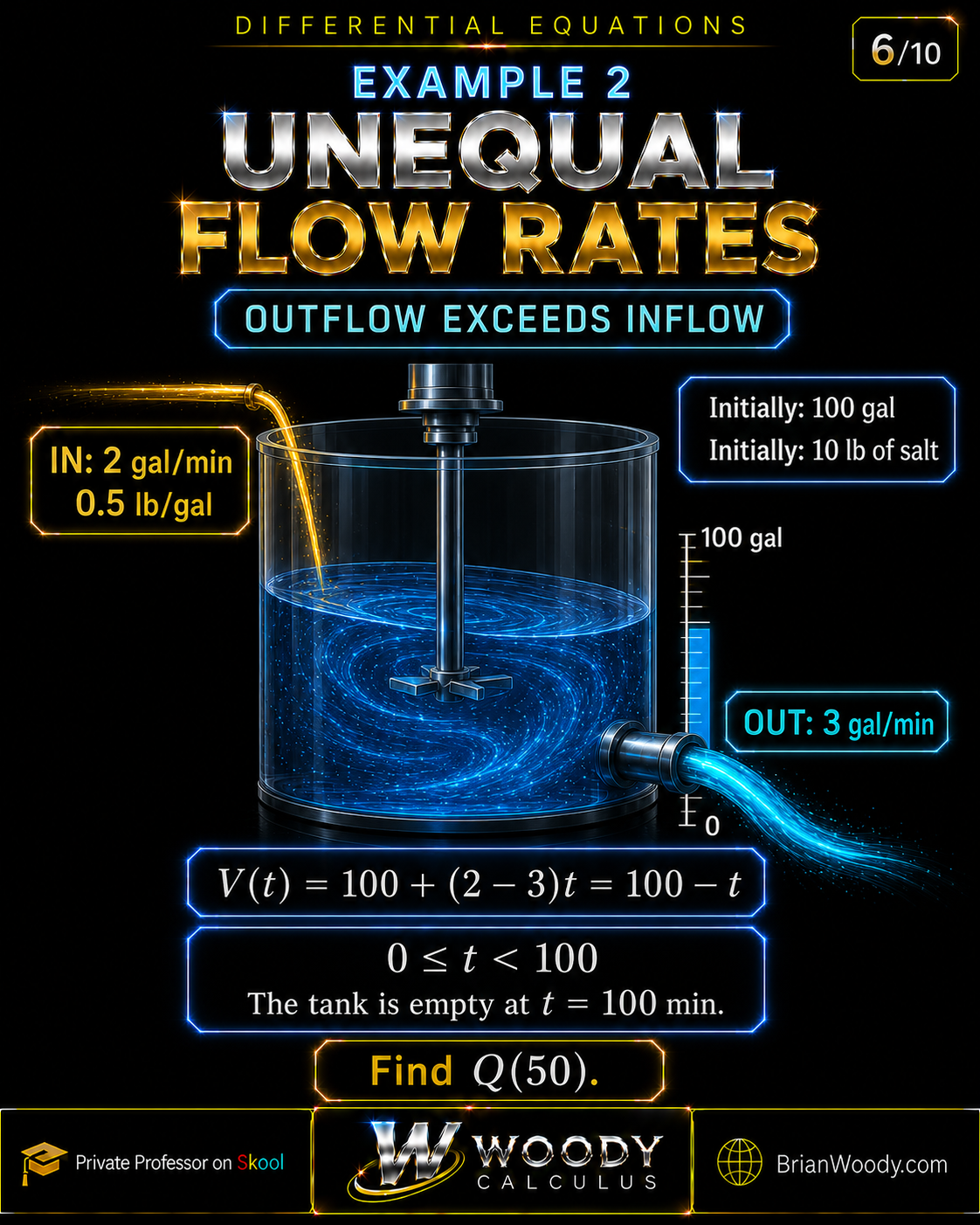
A tank initially contains 100 gallons of solution and 10 pounds of salt. Brine containing 0.5 pound of salt per gallon enters at 2 gallons per minute, while the well-mixed solution leaves at 3 gallons per minute. Find the amount of salt after 50 minutes.
Step 1: Find the physical interval
V(t)=100+(2-3)t=100-t.
\]
The pre-emptying model is valid for
\boxed{0\le t<100}.
\]
Step 2: Build the changing-volume IVP
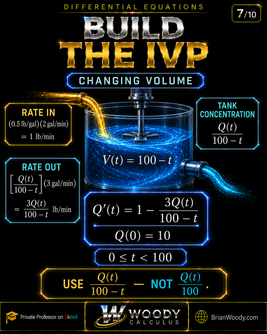
\text{rate in}=(0.5)(2)=1\text{ lb/min},
\]
\[
\text{rate out}=\frac{Q(t)}{100-t}(3)=\frac{3Q(t)}{100-t}\text{ lb/min}.
\]
\boxed{Q^{\prime}=1-\frac{3Q}{100-t},\qquad Q(0)=10.}
\]
Step 3: Solve with a variable integrating factor
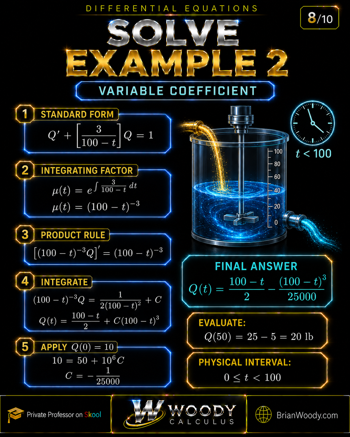
Standard form gives
Q^{\prime}+\frac{3}{100-t}Q=1.
\]
Because \(100-t>0\) on the physical interval,
\mu(t)=e^{\int 3/(100-t)\,dt}
=e^{-3\ln(100-t)}=(100-t)^{-3}.
\]
Multiplying and integrating yields
\bigl((100-t)^{-3}Q\bigr)^{\prime}=(100-t)^{-3},
\]
\[
(100-t)^{-3}Q=\frac{1}{2(100-t)^2}+C,
\]
\[
Q(t)=\frac{100-t}{2}+C(100-t)^3.
\]
Apply \(Q(0)=10\):
10=50+10^6C,
\qquad C=-\frac1{25000}.
\]
\boxed{Q(t)=\frac{100-t}{2}-\frac{(100-t)^3}{25000}},
\qquad 0\le t<100.
\]
Q(50)=25-5=20\text{ lb}.
\]
The hidden maximum amount of salt
The tank is draining, yet the amount of salt initially increases because the incoming salt rate is larger than the initial outgoing salt rate. Differentiate the explicit solution:
Q^{\prime}(t)=-\frac12+\frac{3(100-t)^2}{25000}.
\]
Setting \(Q^{\prime}(t)=0\) gives
t_{\max}=100-\sqrt{\frac{12500}{3}}
\approx35.45\text{ min}.
\]
At this time,
\boxed{Q_{\max}=\frac13\sqrt{\frac{12500}{3}}\approx21.52\text{ lb}}.
\]
The concentration approaches the inflow concentration
Dividing the solution by \(V(t)=100-t\) gives
\frac{Q(t)}{V(t)}
=\frac12-\frac{(100-t)^2}{25000}.
\]
This concentration equals \(0.1\) pound per gallon initially and approaches the incoming concentration:
\lim_{t\to100^-}\frac{Q(t)}{V(t)}=0.5\text{ lb/gal}.
\]
Why \(t=100\) is excluded
The coefficient \(3/(100-t)\) is continuous for \(t<100\), so the linear existence-and-uniqueness theorem applies on intervals that stay below 100. At \(t=100\), the tank is empty and the concentration \(Q/V\) is undefined. The formula has a continuous extension with left-hand limit zero, but the differential-equation model itself ends at the emptying time. See the Existence and Uniqueness Theorem lesson for the interval principle.
Example 3: A Filling Tank That Reaches Overflow
A 100-gallon tank initially contains 50 gallons of solution and 5 pounds of salt. Brine containing 0.2 pound of salt per gallon enters at 3 gallons per minute. The well-mixed solution leaves through an outlet at 2 gallons per minute. Find the amount of salt when the tank reaches capacity.
Step 1: Volume and overflow time
V(t)=50+(3-2)t=50+t.
\]
The tank reaches its 100-gallon capacity when \(50+t=100\), so the pre-overflow model is valid through the capacity time: \(0\le t\le 50\).
Step 2: Build and solve the IVP
\text{rate in}=(0.2)(3)=0.6\text{ lb/min},
\]
\[
\text{rate out}=\frac{Q(t)}{50+t}(2)=\frac{2Q(t)}{50+t}\text{ lb/min}.
\]
\boxed{Q^{\prime}+\frac{2}{50+t}Q=0.6,\qquad Q(0)=5.}
\]
The integrating factor is
\mu(t)=e^{\int2/(50+t)\,dt}=(50+t)^2.
\]
Thus,
\bigl((50+t)^2Q\bigr)^{\prime}=0.6(50+t)^2,
\]
\[
Q(t)=0.2(50+t)+\frac{C}{(50+t)^2}.
\]
Using \(Q(0)=5\) gives \(C=-12500\). Therefore,
\boxed{Q(t)=0.2(50+t)-\frac{12500}{(50+t)^2}},
\qquad 0\le t\le 50.
\]
At the moment the tank reaches capacity,
\boxed{Q(50)=20-1.25=18.75\text{ lb}}.
\]
The concentration at capacity is \(18.75/100=0.1875\) pound per gallon. For \(t>50\), the model must change because an additional well-mixed outflow leaves over the rim.
Equal Flows, Draining Tanks, and Filling Tanks Compared
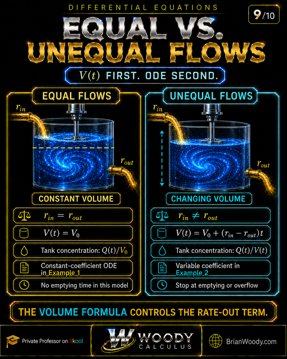
The volume formula determines the outgoing concentration, the ODE coefficient, and the endpoint of the physical model.
| Model | Volume | ODE behavior | Physical endpoint |
|---|---|---|---|
| Equal flows | \(V(t)=V_0\) | Constant coefficient for constant rates | No emptying or overflow from net flow |
| Outflow exceeds inflow | Decreases linearly | Variable coefficient | Stop when the tank empties |
| Inflow exceeds outflow | Increases linearly | Variable coefficient | Stop or change the model at overflow |
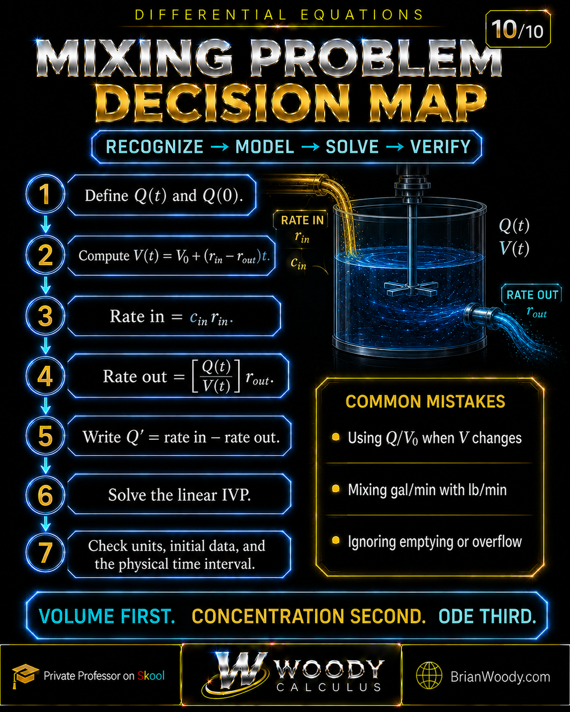
Mixing Problems Decision Map
Use this sequence on homework and exams: recognize the quantities, model the flows, solve the IVP, and verify the physical interpretation.
Define: identify \(Q(t)\), \(Q(0)\), and the units.
Volume: calculate \(V(t)\) and the physical interval.
Rate in: multiply incoming concentration by incoming volumetric flow.
Rate out: multiply the current tank concentration by outgoing volumetric flow.
Model: write \(Q^{\prime}=\text{rate in}-\text{rate out}\).
Solve: use the integrating factor and apply the initial condition.
Verify: check the ODE, units, initial data, sign, and interval.
Common Mixing Problem Mistakes
Most incorrect solutions fail during modeling rather than integration. Check these points before solving.
Using the initial concentration for all time
The tank concentration changes and must be written as \(Q(t)/V(t)\).
Forgetting that the volume changes
When \(r_{\mathrm{in}}\ne r_{\mathrm{out}}\), calculate \(V(t)\) before the rate-out term.
Subtracting volumetric flow from salt rate
Gallons per minute cannot be subtracted from pounds per minute. Convert both substance rates first.
Reversing rate in and rate out
The conservation law is amount rate equals rate in minus rate out.
Losing the integrating-factor sign
For \(3/(100-t)\), substitution gives a negative logarithm and \(\mu=(100-t)^{-3}\).
Ignoring emptying or overflow
An algebraic formula does not extend the physical tank model beyond its valid interval.
Confusing amount with concentration
\(Q(t)\) is an amount; \(Q(t)/V(t)\) is a concentration. Their units are different.
Skipping verification
Substitute into the ODE and initial condition, then check units and physical reasonableness.
Mixing Problems Mastery Check
Try each problem before opening its solution. The set covers constant volume, draining, overflow timing, equilibrium, and modeling logic.
1. Equal flows: solve the IVP and find \(Q(10)\).
An 80-gallon tank initially contains 12 pounds of salt. Brine enters and leaves at 4 gallons per minute, and the inflow concentration is 0.25 pound per gallon.
Solution
The volume is 80 gallons, rate in is 1 pound per minute, and rate out is \(Q/20\). Thus
2. Draining tank: solve the IVP and find \(Q(30)\).
A tank initially contains 60 gallons and 6 pounds of salt. Brine enters at 2 gallons per minute with concentration 0.3 pound per gallon and leaves at 3 gallons per minute.
Solution
Here \(V(t)=60-t\), so \(0\le t<60\), and
The integrating factor is \((60-t)^{-3}\), which gives
3. When does a filling tank reach capacity?
A 120-gallon tank initially contains 70 gallons. Liquid enters at 5 gallons per minute and leaves at 3 gallons per minute.
Solution
Set \(V(t)=120\): \(70+2t=120\), so
The original pre-overflow model is valid through the capacity time, \(0\le t\le25\); for \(t>25\), the model must change.
4. Why is the outgoing concentration \(Q(t)/V(t)\)?
Solution
Perfect mixing makes the concentration uniform throughout the tank. The amount present is \(Q(t)\) and the liquid volume is \(V(t)\), so amount divided by volume is the concentration carried by every outgoing gallon.
5. Find the constant-volume equilibrium amount.
For constant volume \(V_0\), constant inflow concentration \(c_{\mathrm{in}}\), and equal flow rate \(r\), determine the equilibrium amount.
Solution
Set \(Q^{\prime}=0\) and cancel \(r>0\):
Mixing Problems Glossary
These definitions connect the physical tank model with the first-order differential equation.
- Mixing problem
- A differential-equation model that tracks the amount of a substance entering, leaving, and remaining in a well-mixed container.
- Perfect mixing
- The assumption that concentration is uniform throughout the tank at each time.
- Rate in
- Incoming concentration multiplied by incoming volumetric flow rate.
- Rate out
- Current tank concentration multiplied by outgoing volumetric flow rate.
- Constant volume
- The case in which equal volumetric inflow and outflow keep \(V(t)=V_0\).
- Changing volume
- The case in which unequal volumetric flow rates make \(V(t)\) depend on time.
- Integrating factor
- The multiplier \(\mu(t)=e^{\int P(t)\,dt}\) used to solve a linear equation \(Q^{\prime}+P(t)Q=g(t)\).
- Physical interval
- The time interval during which the tank assumptions, volume, and specified flow configuration remain valid.
- Equilibrium amount
- A constant amount \(Q_{\mathrm{eq}}\) for which rate in equals rate out and \(Q^{\prime}=0\).
- Initial-value problem
- A differential equation together with initial data such as \(Q(0)=Q_0\).
Frequently Asked Questions About Mixing Problems
These concise answers summarize the model, volume calculation, integrating-factor method, and physical restrictions.
What is a mixing problem in differential equations?
A mixing problem tracks the amount of a dissolved substance in a well-mixed tank. The governing balance is amount rate equals rate in minus rate out.
What is the basic differential equation for a mixing problem?
If \(Q(t)\) is the amount, \(V(t)\) is the volume, \(c_{\mathrm{in}}\) is the incoming concentration, and \(r_{\mathrm{in}},r_{\mathrm{out}}\) are the flow rates, then \(Q^{\prime}(t)=c_{\mathrm{in}}r_{\mathrm{in}}-[Q(t)/V(t)]r_{\mathrm{out}}\).
Why is the outgoing concentration Q(t)/V(t)?
Perfect mixing makes the concentration uniform throughout the tank. Amount divided by volume is therefore the concentration carried by the outgoing solution.
How do you calculate the volume in a mixing problem?
For constant flow rates, use \(V(t)=V_0+(r_{\mathrm{in}}-r_{\mathrm{out}})t\). Then restrict time so the volume stays positive and does not exceed tank capacity.
What happens when the inflow and outflow rates are equal?
The volume remains constant. With constant concentrations and flow rates, the resulting first-order linear ODE has a constant coefficient.
What happens when the inflow and outflow rates are different?
The volume changes with time, so the outgoing concentration and the coefficient of the linear ODE usually depend on time. The model must stop or change when the tank empties or overflows.
How do you solve the linear ODE in a mixing problem?
Write the equation as \(Q^{\prime}+P(t)Q=g(t)\), compute the integrating factor \(\mu(t)=e^{\int P(t)dt}\), integrate the product equation, and apply the initial condition.
When must a tank mixing model stop?
Stop at the first time the tank becomes empty or reaches capacity unless the problem explicitly supplies a new flow configuration after that event.
What is the difference between amount and concentration?
Amount \(Q(t)\) is measured in units such as pounds or grams. Concentration \(Q(t)/V(t)\) is measured in amount per unit volume, such as pounds per gallon.
How do you check a mixing problem answer?
Verify the differential equation and initial condition, confirm that every rate has compatible units, check that amounts and volumes are physically meaningful, and respect the valid time interval.
References and Further Study
This lesson follows the standard undergraduate treatment of first-order linear differential equations and compartment mixing models.
- Dennis G. Zill, A First Course in Differential Equations with Modeling Applications, 12th edition, Cengage, 2024.
- William E. Boyce, Richard C. DiPrima, and Douglas B. Meade, Elementary Differential Equations and Boundary Value Problems, 12th edition, Wiley, 2021.
- C. Henry Edwards, David E. Penney, and David Calvis, Differential Equations and Boundary Value Problems: Computing and Modeling, 6th edition, Pearson, 2022.
Continue Learning Differential Equations
Use these Woody Calculus lessons to strengthen first-order method selection, theory, visualization, and numerical approximation.