Differential Equations • Woody Calculus
Second-order linear differential equations become dramatically easier when you stop seeing them as a collection of unrelated formulas and start seeing the root structure underneath them. For a homogeneous equation with constant coefficients, one quadratic equation—the characteristic equation—determines the entire shape of the general solution.
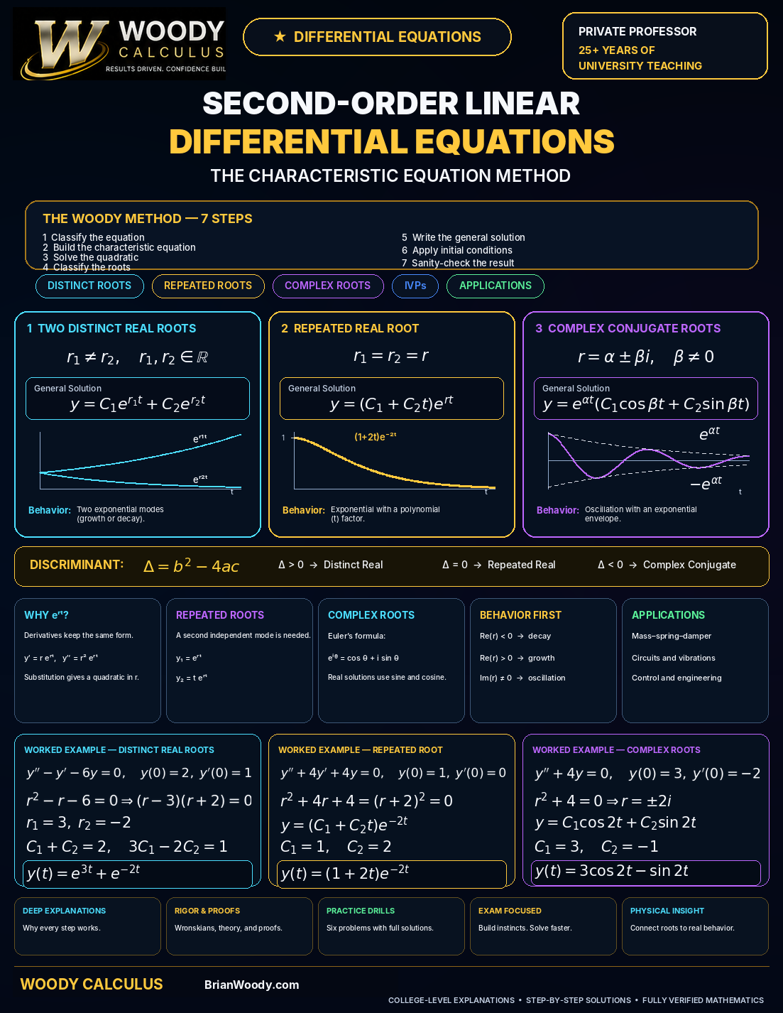
In plain English: classify the equation, form the characteristic quadratic, solve for its roots, match the root type to the correct general-solution template, and apply initial conditions only after the general solution is correct.
When Can You Use the Characteristic Equation?
The standard characteristic-equation method in this lesson applies directly to a very specific class of differential equations:
where are constants and .
Classify the equation before you solve it
| Equation | Use the ordinary characteristic equation directly? | Why? |
|---|---|---|
| YES | Second-order, linear, homogeneous, constant coefficients. | |
| NO | Variable coefficients. This is a Cauchy–Euler type equation, which uses a different substitution. | |
| PARTLY | The characteristic equation finds the homogeneous part , but another method is needed for a particular solution. | |
| NO | Nonlinear because multiplies . |
Why Do We Try an Exponential Solution?
The characteristic equation is not a random trick. Exponentials are special because differentiation preserves their form.
Each derivative changes only the algebraic multiplier in front of the same exponential function. That is exactly what we need: a differential equation can collapse into a polynomial equation in .
we obtain
Factor out the common exponential:
Because for real , the only way the product can vanish is
What Is the Characteristic Equation?
You may also see the phrases auxiliary equation or characteristic polynomial. The roots of this quadratic are the characteristic roots.
The important idea is not merely that we solve a quadratic. The root structure tells us which pair of linearly independent solution modes spans the two-dimensional solution space.
Why Are There Exactly Two Arbitrary Constants?
This is the normalized form of a general linear equation. If one begins with , the theorem applies on any interval where and the normalized coefficient functions are continuous.
For the homogeneous equation, this theorem explains the two-dimensional solution space. Two linearly independent solutions form a basis, so every solution has the form
The two constants are not decorative. They encode the two independent pieces of initial data: position and velocity. For constant coefficients, the normalized coefficient functions are continuous everywhere, so the theorem applies on the entire real line.
Why Two Independent Solution Modes Matter
The characteristic equation does not merely hand us isolated solutions. It identifies a basis for the entire homogeneous solution space.
For a second-order equation, two linearly independent solutions are enough to produce the general homogeneous solution. This is why the characteristic equation must ultimately give us two independent modes—even when it produces only one numerical root.
What does “linearly independent” mean here?
Two solutions are linearly independent if one is not merely a constant multiple of the other. If , then
so the supposed two-constant family is actually only one-dimensional. That is exactly the problem repeated roots create and exactly why the extra factor matters.
The Wronskian is the fast independence test
For two differentiable functions, define
If the Wronskian is nonzero at some point on the interval, the two functions are linearly independent. Moreover, when both functions solve the same linear homogeneous second-order ODE, Abel’s identity implies that a Wronskian that is nonzero at one point cannot suddenly vanish elsewhere on the interval. For distinct exponential roots,
which is nonzero whenever . That is the structural reason two distinct roots automatically produce two independent solution modes.
Quadratic Formula and the Discriminant
Factoring is convenient, but the method does not depend on a nice factorization. The characteristic roots always come from the quadratic formula:
Define the discriminant
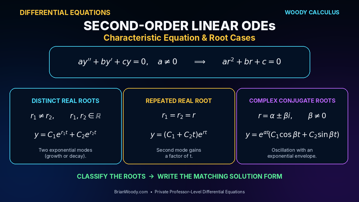
Then the sign of tells you the root type before you even finish simplifying the roots:
For a negative discriminant, write
and identify the real and imaginary parts of the roots. This is usually faster and safer than trying to force a factorization that does not exist over the real numbers.
The Three Root Cases You Must Recognize
For the quadratic characteristic equation, everything is controlled by the discriminant
| Root type | Discriminant | General solution | Main behavior |
|---|---|---|---|
| Two distinct real roots | Two exponential modes | ||
| Repeated real root | Repeated exponential mode with a new independent solution | ||
| Complex conjugate roots | Oscillation with exponential envelope |
Case 1: Two Distinct Real Roots
Consider the initial-value problem
The roots are real and distinct, so the general solution is
From ,
Differentiate:
Using ,
Solving the two equations gives and .
Case 2: A Repeated Real Root
Now solve
The characteristic equation is
so there is one repeated root:
The correct second independent solution is , giving
Use to get . Differentiate:
Then gives , so .
Why Do Repeated Roots Require Multiplying by t?
This is one of the most memorized and least explained rules in elementary Differential Equations. There are two facts to understand.
1. We need two linearly independent solutions
If is a repeated root, gives one solution. Another constant multiple of the same function does not create a second direction in the solution space.
2. The function t ert is actually another solution
For ,
Substituting into the differential operator gives
For a repeated root, both
hold, because a double root makes both the characteristic polynomial and its derivative vanish. Therefore solves the ODE.
The Wronskian confirms independence
So and really do form two independent solution modes.
Case 3: Complex Conjugate Roots
Consider
The characteristic equation is
Using Euler’s formula, complex exponentials can be converted into real sine and cosine modes. The real general solution is
From , we get . Differentiate:
Using ,
The general complex-root formula
If the characteristic roots are
then the real general solution is
The real part controls exponential growth or decay, while the imaginary magnitude controls oscillation frequency.
Therefore
Decaying oscillation
Why Do Complex Roots Produce Sine and Cosine?
The appearance of trigonometric functions is not a separate rule pasted onto the characteristic-equation method. It comes directly from Euler’s formula.
Suppose the characteristic equation has the real-coefficient roots
Because the coefficients are real, nonreal roots occur as a conjugate pair. One complex exponential mode is
Euler’s formula says
Therefore
Write the complex solution as . Because the differential operator has real coefficients, applying it gives . If the complex output is zero, both its real and imaginary parts are zero. Therefore the real and imaginary parts separately provide real solutions:
That is why the complex-root template is
Amplitude–Phase Form: One Cosine With an Amplitude and Phase Shift
The complex-root solution is often written as a sine-cosine combination, but many applications and exams ask for a single shifted cosine.
Choose
If , use the quadrant-correct phase rather than a one-argument arctangent that can choose the wrong quadrant. If , then the solution is identically zero and the phase is irrelevant.
Then the general complex-root solution can be written as
Envelope amplitude
The nonnegative number is the amplitude of the exponential envelope at . The actual initial displacement is .
Phase shift
The angle controls where the oscillation begins in its cycle.
When , the amplitude envelope is , so the oscillation decays while its frequency remains controlled by .
Special Root Cases Students Often Miss
A characteristic root can be zero
Consider
The characteristic equation is
The roots are and . Since , the constant function is one of the modes:
A zero root is not a special fourth template. It is simply the distinct-real-root formula with one exponential equal to one.
A double zero root produces a linear function
If the equation is
then the characteristic equation is , a repeated root at zero. The repeated-root template gives
That agrees perfectly with integrating twice. This is a useful sanity check on the repeated-root rule.
What if a = 0?
If the coefficient of is zero, the equation is no longer second order. Do not mechanically write a quadratic characteristic equation when the differential equation itself has dropped to first order.
Initial Conditions Do Not Have to Be at t = 0
Textbook examples often use because the exponentials simplify, but the method works at any initial point.
Consider
From the roots and ,
The derivative condition gives
Then gives , so . A clean final form is
The lesson is procedural: the initial point changes the algebra, not the root classification.
Initial-Value Problems vs. Boundary-Value Problems
Initial-value problem
Both conditions are specified at the same point:
Under the standard continuity assumptions, these data determine one unique solution.
Boundary-value problem
Conditions are imposed at different points, for example
The characteristic equation still gives the general homogeneous solution, but the boundary conditions may produce one solution, no solution, or multiple solutions.
This distinction matters later in eigenvalue problems, Fourier series, heat equations, wave equations, and Sturm–Liouville theory.
How Do You Verify a Characteristic-Equation Solution?
Verification is especially valuable while you are learning the templates. There are three layers to check.
Differentiate the proposed solution and substitute it into the left side of the ODE.
Evaluate and directly.
Make sure the number and type of modes agree with the characteristic roots.
For the earlier solution
we have
Substitute into :
Both exponential coefficients cancel exactly. Verification is also a quick way to catch sign errors in the characteristic roots.
What Do Characteristic Roots Tell You About Solution Behavior?
The roots do more than produce a formula. They reveal the qualitative modes before you finish an initial-value problem.
| Root information | Mode behavior |
|---|---|
| Real root | The mode decays as . |
| Real root | The mode grows exponentially as . |
| Roots with | Oscillations decay under the envelope . |
| Roots | Persistent undamped sinusoidal oscillation. |
| Roots with | Oscillations grow exponentially. |
For a linear combination of several modes, the term associated with the root having the largest real part generally controls long-term behavior unless its coefficient happens to be zero.
This perspective connects naturally to the Woody Calculus lessons on phase portraits and stability and eigenvalues and eigenvectors.
Spring–Mass–Damper Systems: The Discriminant Becomes Physics
A standard mechanical model is
with mass , damping coefficient , and spring constant . The characteristic equation is
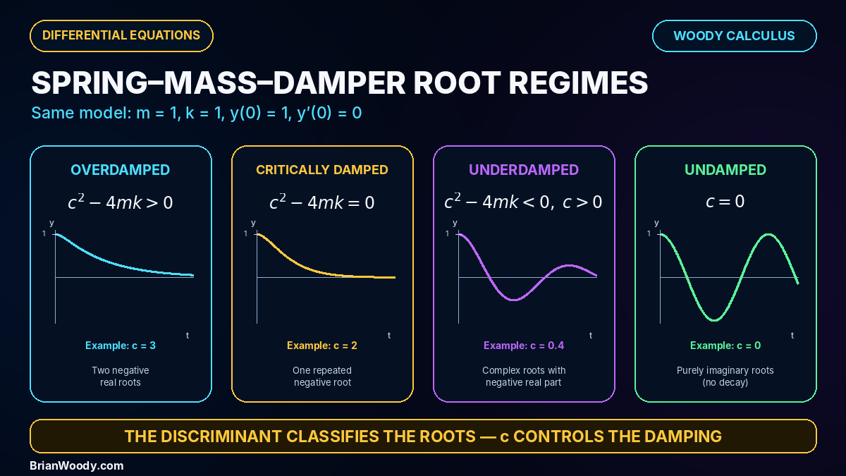
When , the discriminant separates the three damped regimes. The special case is undamped.
| Condition | Root type | Mechanical regime |
|---|---|---|
| Two distinct real roots | Overdamped | |
| Repeated real root | Critically damped | |
| Complex roots with negative real part | Underdamped | |
| Pure imaginary roots | Undamped |
For forced oscillations and resonance, continue with Resonance in Differential Equations.
Characteristic Equation vs. Eigenvalue Equation
Students often notice that the algebra looks familiar. In a scalar second-order ODE, the characteristic equation is
For a matrix system, eigenvalues satisfy
These are not the same equation, but they express the same broad structural idea: special algebraic values identify the fundamental solution modes of a linear dynamical system.
This connection becomes explicit when higher-order scalar ODEs are rewritten as first-order systems. See Eigenvalues and Eigenvectors Explained and Systems of Differential Equations Help.
When the Characteristic Equation Is Not Enough
For a nonhomogeneous equation
the characteristic equation still gives the homogeneous solution , but that is only part of the answer. The full solution has the form
The particular solution requires another method. Depending on the forcing function and course context, that may be the method of undetermined coefficients, variation of parameters, or a Laplace transform.
Which Second-Order Differential Equation Method Should You Use?
The characteristic equation is one tool inside a larger second-order ODE toolbox. A strong Differential Equations student recognizes the equation class before choosing the method.
| Equation / goal | Primary method | What the method gives |
|---|---|---|
| , constant coefficients | Characteristic equation | Complete homogeneous solution from the roots. |
| with suitable polynomial/exponential/trig forcing | Undetermined coefficients | A trial particular solution , combined with . |
| General linear nonhomogeneous second-order equation once a fundamental homogeneous pair is known | Variation of parameters | A particular solution using integrals built from the homogeneous modes. |
| Initial-value problem with discontinuous or piecewise forcing | Laplace transforms | An algebraic equation in the transform domain, then inverse transform. |
| Variable-coefficient equation near an ordinary point | Power series | A local series solution determined recursively. |
Notice the recurring architecture: even when another method is required, the homogeneous characteristic roots often remain the first piece of the solution.
The Operator-Factorization View: Why the Roots Behave Like Modes
If denotes differentiation with respect to , then
Suppose the characteristic polynomial factors as
Then the differential operator factors analogously:
Because these are constant-coefficient differential operators, the factors commute:
Therefore either modal factor may be applied first. This commutativity is one reason the constant-coefficient method is so clean; variable-coefficient operator factors generally do not commute.
The exponential is killed by because
Likewise is killed by . This factorization viewpoint explains why the roots of the algebraic polynomial correspond so directly to the natural modes of the differential equation.
What changes for a repeated root?
If the polynomial contains , the operator contains . One mode is ; the generalized second mode is . This is the scalar ODE analogue of what later appears in Linear Algebra when repeated eigenvalues lead to generalized eigenvectors and Jordan chains.
How Does the Characteristic Equation Extend to Higher-Order ODEs?
The same architecture extends beyond second order. For a homogeneous constant-coefficient equation
the exponential trial produces the degree- characteristic polynomial
A real root of multiplicity contributes the chain
So the second-order repeated-root rule is not an isolated exception. It is the first nontrivial case of a general multiplicity pattern.
Second-Order Linear ODE Quick Reference
Characteristic equation:
Three cases:
Exam rule: roots first, template second, initial conditions last.
The Woody Calculus Decision Method for Characteristic Equations
Under exam pressure, you want a repeatable classification system—not improvisation.
Confirm that you have a second-order linear homogeneous equation with constant coefficients.
Replace the derivative structure by powers of : .
Factor when convenient or use the quadratic formula.
Distinct real, repeated real, or complex conjugate.
Do not touch the initial conditions until this structure is correct.
Differentiate carefully, substitute the initial data, and solve for .
Verify the root type, count two independent constants before applying initial data, and substitute back when the algebra is short enough.
Common Characteristic-Equation Mistakes
Practice Problems: Characteristic Equation and Root Classification
Try each problem before opening the solution. Say the root classification aloud before you write the solution template.
Problem 1 — Distinct real roots: Solve y″ − 5y′ + 6y = 0.
Roots: . Therefore
Problem 2 — Repeated root: Solve y″ + 6y′ + 9y = 0.
Repeated root . Therefore
Problem 3 — Pure imaginary roots: Solve y″ + 9y = 0.
Problem 4 — General complex roots: Solve y″ + 4y′ + 13y = 0.
Problem 5 — Initial-value problem: Solve y″ − y′ − 6y = 0 with y(0)=2 and y′(0)=1.
The roots are and , so
The initial conditions give and , so .
Problem 6 — Method recognition: Which equations can the ordinary characteristic-equation method solve directly?
A. — Yes.
B. — No. Variable coefficient.
C. — Not for the full solution. It gives ; another method is required for .
D. — No. Nonlinear.
E. — Yes.
F. — Not by the ordinary constant-coefficient method. It is a Cauchy–Euler type equation.
Second-Order Linear Differential Equations FAQ
What is the characteristic equation in Differential Equations?
For a homogeneous second-order linear ODE with constant coefficients , the characteristic equation is . Its roots determine the form of the general solution.
Why do we try an exponential solution?
Because derivatives of an exponential preserve the same exponential factor. Substitution converts derivatives into powers of , reducing the ODE to an algebraic polynomial equation.
When can I use the characteristic-equation method?
The standard method here applies directly to linear homogeneous ODEs with constant coefficients. For a nonhomogeneous equation, it still finds the homogeneous solution but not the particular solution.
What is the solution for two distinct real roots?
If the roots are , then .
What is the solution for a repeated root?
If the characteristic equation has a double root , then .
Why do repeated roots require multiplying by t?
A repeated root gives only one exponential mode . The factor produces a second linearly independent solution , whose Wronskian with is nonzero.
What is the solution for complex roots?
If the roots are , then the real general solution is .
What does the discriminant tell you?
For , gives two distinct real roots, equality gives a repeated real root, and a negative discriminant gives complex conjugate roots.
Why are there two constants C1 and C2?
A homogeneous linear second-order equation has a two-dimensional solution space, so its general solution requires two linearly independent solution modes and two arbitrary constants.
When should initial conditions be applied?
After the root type has been identified and the correct general solution has been written. Applying initial conditions too early is a common source of errors.
Does the characteristic equation solve a nonhomogeneous differential equation?
Not by itself. It gives the homogeneous part . A particular solution must be found by another method such as undetermined coefficients, variation of parameters, or Laplace transforms.
How do characteristic roots relate to damping?
For a spring–mass–damper equation , the discriminant separates the overdamped, critically damped, and underdamped cases when . When , the motion is undamped.
How are characteristic roots related to eigenvalues?
Both characteristic roots and eigenvalues identify fundamental modes of linear systems. A second-order scalar ODE can be rewritten as a first-order system, where the same modal behavior appears through matrix eigenvalues.
What does the existence–uniqueness theorem add to this method?
For the normalized equation, if are continuous on an interval containing , then one position value and one velocity value determine exactly one solution on that interval. This theorem explains why the homogeneous solution space needs two independent modes and two arbitrary constants.
How do you convert sine and cosine into amplitude–phase form?
Write as , where , , and .
What is the difference between an initial-value problem and a boundary-value problem?
An initial-value problem specifies the function and its derivative at the same point. A boundary-value problem imposes conditions at different points. The characteristic equation supplies the general homogeneous solution in both settings, but boundary conditions may produce one solution, no solution, or multiple solutions.
University-Level References
Turn the Root Classification Into Exam-Ready Skill
The fastest way to become reliable with second-order equations is to make the classification automatic: identify the equation type, form the characteristic equation, classify the roots, write the correct solution template, and only then apply initial conditions.
Differential Equations Help
Join the Woody Calculus Mastery Lab
Explore the Math Library