DIFFERENTIAL EQUATIONS • SECOND-ORDER IVPs • STEPS • IMPULSES • CONVOLUTION
Laplace transforms turn a second-order differential equation into algebra while carrying the initial conditions with them. That single idea gives one systematic method for ordinary forcing, piecewise inputs, delayed switches, short impulses, and convolution.
This lesson begins with the derivative formulas, solves one complete initial-value problem without skipping algebra, and then builds the deeper structure: transfer functions, step responses, impulse responses, and convolution. Use it as a first lesson, an exam reference, or a complete map of the Laplace-transform chapter.
Reading time: approximately 55–70 minutes for the complete lesson; 10–15 minutes for the direct answer, algorithm, and worked example.
How Do You Solve a Second-Order ODE with Laplace Transforms?
For a constant-coefficient initial-value problem
a y^{\prime\prime}+b y^{\prime}+cy=f(t),
\qquad y(0)=y_0,
\qquad y^{\prime}(0)=y_1,
\]
define \(Y(s)=\mathcal L\{y(t)\}\) and \(F(s)=\mathcal L\{f(t)\}\). The derivative identities
\mathcal L\{y^{\prime}\}=sY-y_0,
\qquad
\mathcal L\{y^{\prime\prime}\}=s^2Y-sy_0-y_1
\]
convert the differential equation into an algebraic equation. Solving once for \(Y(s)\) gives the master formula
\boxed{
Y(s)=\frac{F(s)+asy_0+ay_1+by_0}{as^2+bs+c}
}.
\]
Factor the denominator, use partial fractions or another inverse-transform technique, and apply \(\mathcal L^{-1}\) term by term. For delayed inputs, \(e^{-as}\) means a time delay; for an impulse at \(t=a\), \(\mathcal L\{\delta(t-a)\}=e^{-as}\); and when \(Y(s)=F(s)H(s)\), the time-domain response is the convolution \(y=f*h\).
Quick Summary
- Laplace transforms replace differentiation in \(t\) with multiplication by \(s\), plus explicit initial-data terms.
- The quadratic \(as^2+bs+c\) is the transformed differential operator and controls the natural modes, poles, transients, and stability.
- The numerator combines the external input \(F(s)\) with the initial conditions.
- Partial fractions convert rational expressions into recognizable inverse-transform pieces.
- A factor \(e^{-as}\) means the time-domain response is delayed until \(t=a\).
- The unit step \(u(t-a)\) turns a forcing term on at \(t=a\); a difference of steps creates a finite pulse.
- The Dirac delta \(\delta(t-a)\) represents an idealized impulse concentrated at one time.
- The impulse response is \(h(t)=\mathcal L^{-1}\{1/(as^2+bs+c)\}\).
- For zero initial conditions, the output to an arbitrary input is \(y=f*h\).
- Laplace transforms are systematic, especially for IVPs, switching, piecewise forcing, and impulses, but they are not always the shortest method.
Memory sentence: Operator to denominator; input plus initial data to numerator; factor, invert, and verify.
The Seven-Step Laplace Transform Algorithm
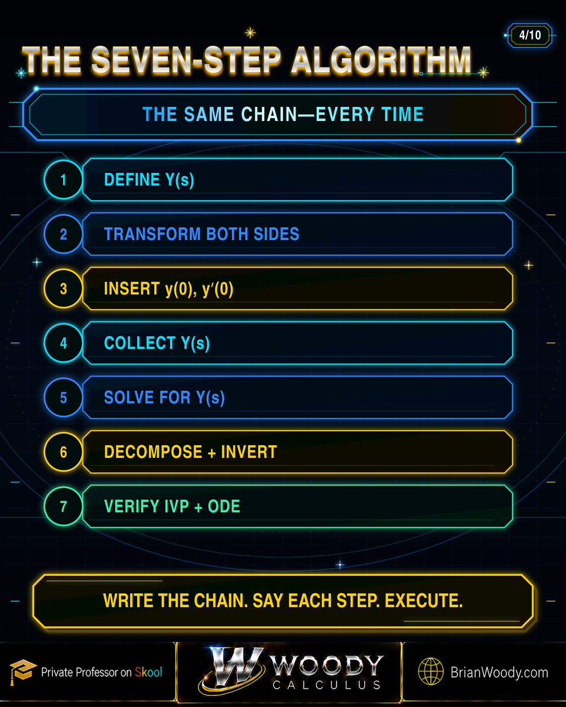
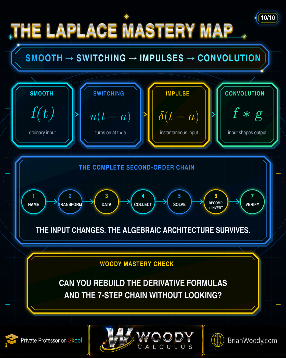
- Define the transformed unknown. Write Y(s) = L{y(t)} so every transformed derivative can be expressed in terms of one function.
- Transform both sides. Apply linearity and transform each derivative and forcing term separately.
- Insert the initial data immediately. Substitute y(0) and y prime(0) before collecting Y(s).
- Collect every Y(s) term. Factor Y(s) from the transformed differential operator.
- Solve algebraically for Y(s). Factor the denominator completely and simplify the numerator.
- Decompose and invert. Use partial fractions, shifting rules, convolution, or a transform table to recover y(t).
- Verify the initial-value problem. Check both initial conditions and substitute the result into the original differential equation on every relevant time interval.
Table of Contents
- The Laplace architecture for second-order equations
- Definition, existence, and the transform table
- The derivative engine and master formula
- The seven-step method
- Complete worked IVP from start to finish
- Partial fractions and inverse-transform patterns
- Unit step functions and delayed forcing
- Complete switched-input example
- Dirac delta impulses and jump behavior
- Convolution and the impulse-response formula
- Transfer functions, poles, transients, and steady state
- Method selection, checks, and common mistakes
- Mastery map and practice set
- Frequently asked questions
Part I — The Laplace Architecture for Second-Order Equations
The central translation: derivatives become algebra
A differential equation describes how a function changes. That is ideal for modeling but can be awkward for calculation because the unknown \(y\), its derivatives, the forcing input, and the initial conditions appear in different forms. The Laplace transform translates all of them into functions of a new variable \(s\).
In the \(t\)-domain, the equation
a y^{\prime\prime}+b y^{\prime}+cy=f(t)
\]
is a relationship among derivatives. In the \(s\)-domain it becomes
(as^2+bs+c)Y(s)=F(s)+asy_0+ay_1+by_0.
\]
The unknown is no longer being differentiated. It is multiplied by a quadratic polynomial. The initial conditions have not been postponed or discarded; they appear as concrete numerator terms.
Operator, input, and data
Operator
\(aD^2+bD+c\) becomes \(as^2+bs+c\). This denominator contains the natural modes of the system.
Input
\(f(t)\) becomes \(F(s)\). Smooth, switched, pulsed, and impulsive inputs enter through the same algebraic channel.
Initial data
\(y_0\) and \(y_1\) become numerator terms. They describe the response already stored in the system at \(t=0\).
Zero-input and zero-state responses
The master formula naturally separates the solution into two parts:
Y(s)=
\underbrace{\frac{asy_0+ay_1+by_0}{as^2+bs+c}}_{\text{response to initial data}}
+
\underbrace{\frac{F(s)}{as^2+bs+c}}_{\text{response to the external input}}.
\]
The first part is called the zero-input response: set the external input to zero but retain the initial state. The second is the zero-state response: set the initial conditions to zero but retain the forcing. This split later becomes the cleanest route to convolution.
The mass-spring-damper model behind the symbols
A standard physical example is
m y^{\prime\prime}+d y^{\prime}+ky=F(t).
\]
Here \(m\) is mass, \(d\) is damping, \(k\) is stiffness, \(F(t)\) is the applied force, \(y\) is displacement, and \(y^{\prime}\) is velocity. The two initial values describe the displacement and velocity already present when observation begins.
In the transform domain,
(ms^2+ds+k)Y(s)=F(s)+msy_0+my_1+dy_0.
\]
The denominator is the system itself. Changing the applied force changes \(F(s)\), but it does not change the system denominator. This is why one transfer function can be reused for a step, a pulse, an impulse, or a completely general input.
What class of problems fits this method best?
The clean algebraic workflow in this lesson is designed for linear constant-coefficient IVPs on \(t\ge0\). Laplace transforms can also handle some variable-coefficient equations and integral equations, but multiplication by \(t\) produces derivatives with respect to \(s\), so the transformed problem may remain differential rather than algebraic. The method is most efficient when the coefficients are constant and the forcing has a known transform or a useful convolution representation.
Part II — Definition, Existence, and the Essential Transform Table
The Laplace transform of a function \(f(t)\), defined for \(t\ge0\), is
\mathcal L\{f(t)\}=F(s)=\int_0^{\infty}e^{-st}f(t)\,dt,
\]
for values of \(s\) where the improper integral converges. The factor \(e^{-st}\) suppresses sufficiently moderate growth as \(t\to\infty\). A standard sufficient condition is that \(f\) be piecewise continuous on every finite interval and of exponential order: \(|f(t)|\le Me^{\alpha t}\) for sufficiently large \(t\). These are convenient guarantees, not the most general possible conditions.
Why the one-sided transform fits initial-value problems
The integral begins at \(t=0\), exactly where the initial conditions are supplied. That makes the one-sided Laplace transform a natural tool for causal systems: the input starts at \(t=0\), a switch occurs later at \(t=a\), and an impulse is applied at a specified time.
Essential Laplace transform table
| Time-domain function | Laplace transform | Use |
|---|---|---|
| \(1\) | \(1/s\) | Constant inputs and steady values |
| \(t^n\) | \(n!/s^{n+1}\) | Polynomial forcing |
| \(e^{at}\) | \(1/(s-a)\) | Exponential modes |
| \(\cos bt\) | \(s/(s^2+b^2)\) | Oscillatory forcing |
| \(\sin bt\) | \(b/(s^2+b^2)\) | Oscillatory forcing |
| \(e^{at}f(t)\) | \(F(s-a)\) | First shifting theorem |
| \(u(t-a)f(t-a)\) | \(e^{-as}F(s)\) | Delayed inputs |
| \(\delta(t-a)\) | \(e^{-as}\) | Idealized impulse at \(t=a\) |
| \((f*g)(t)\) | \(F(s)G(s)\) | Arbitrary-input response |
Linearity keeps the workflow manageable
\mathcal L\{\alpha f+\beta g\}=\alpha F+\beta G.
\]
Linearity lets us transform a differential equation term by term. The difficult structural work is concentrated in three places: derivative formulas, algebraic simplification, and inversion.
Four additional transform rules worth knowing
| Time-domain operation | Transform-domain result | Interpretation |
|---|---|---|
| Multiply by \(e^{at}\) | \(\mathcal L\{e^{at}f(t)\}=F(s-a)\) | Shift the transform horizontally |
| Multiply by \(t\) | \(\mathcal L\{tf(t)\}=-F^{\prime}(s)\) | Useful for repeated-pole inversions |
| Integrate in time | \(\mathcal L\{\int_0^t f(\tau)d\tau\}=F(s)/s\) | Explains why step response accumulates impulse response |
| Convolve | \(\mathcal L\{f*g\}=F(s)G(s)\) | Turns a time integral into multiplication |
Why matching transforms gives the solution
Under the usual piecewise-continuity and exponential-order hypotheses, the Laplace transform is unique up to equality at isolated points. Once the algebra produces a valid \(Y(s)\), its inverse identifies the causal time-domain solution. That uniqueness is what makes transform tables and partial fractions legitimate solution tools rather than pattern-matching guesses.
Part III — The Derivative Engine and the Master Formula
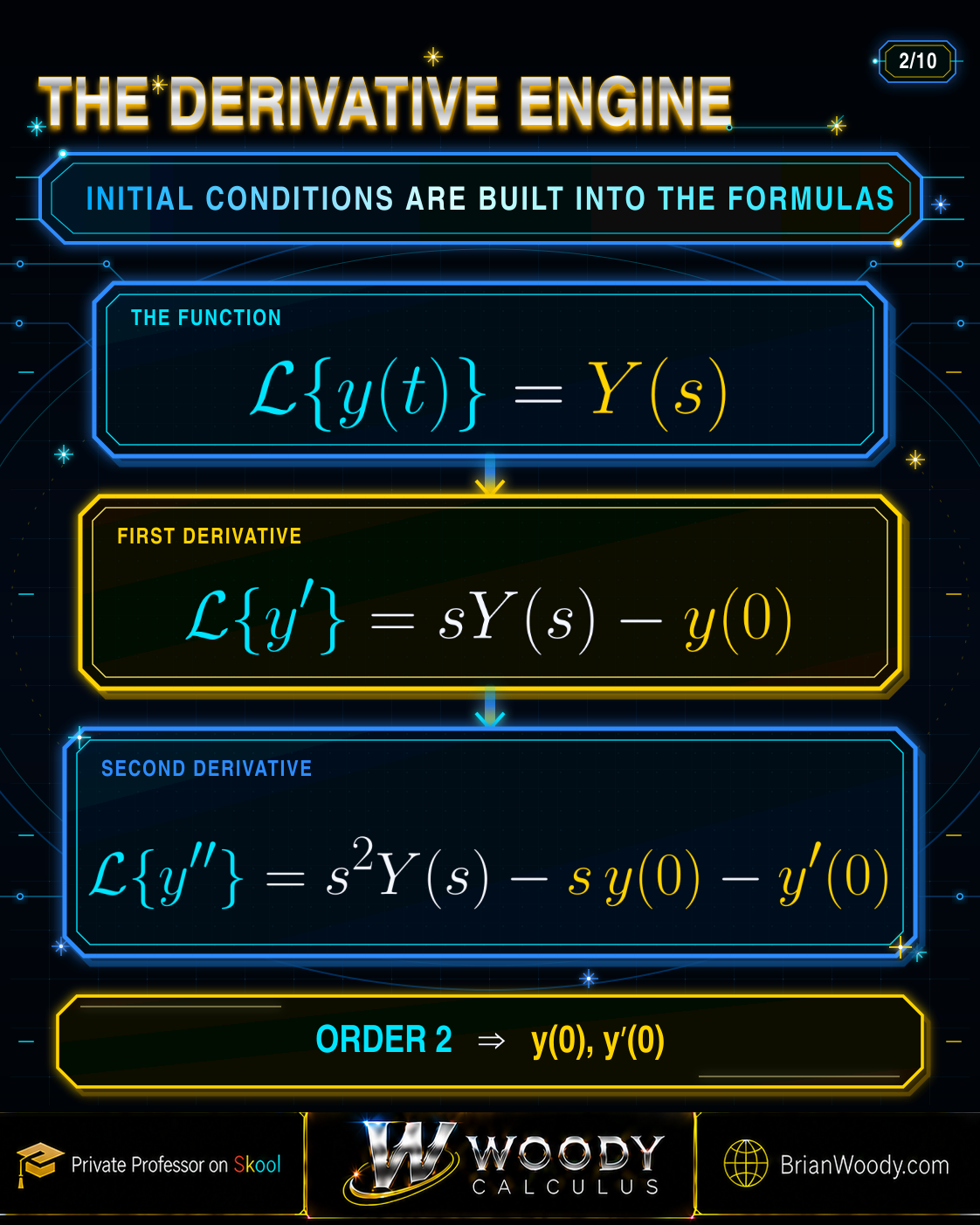
First derivative
Integration by parts gives
\mathcal L\{y^{\prime}\}=sY(s)-y(0).
\]
The term (-y(0)) is not an inconvenience. It is the mechanism that inserts the first initial condition into the transformed problem.
Second derivative
Apply the first-derivative formula again:
\begin{aligned}
\mathcal L\{y^{\prime\prime}\}
&=s\mathcal L\{y^{\prime}\}-y^{\prime}(0)\\
&=s\bigl(sY-y(0)\bigr)-y^{\prime}(0)\\
&=s^2Y-sy(0)-y^{\prime}(0).
\end{aligned}
\]
A second-order equation therefore requires two initial values. In general,
\mathcal L\{y^{(n)}\}
=s^nY-s^{n-1}y(0)-s^{n-2}y^{\prime}(0)-\cdots-y^{(n-1)}(0).
\]
Deriving the master formula
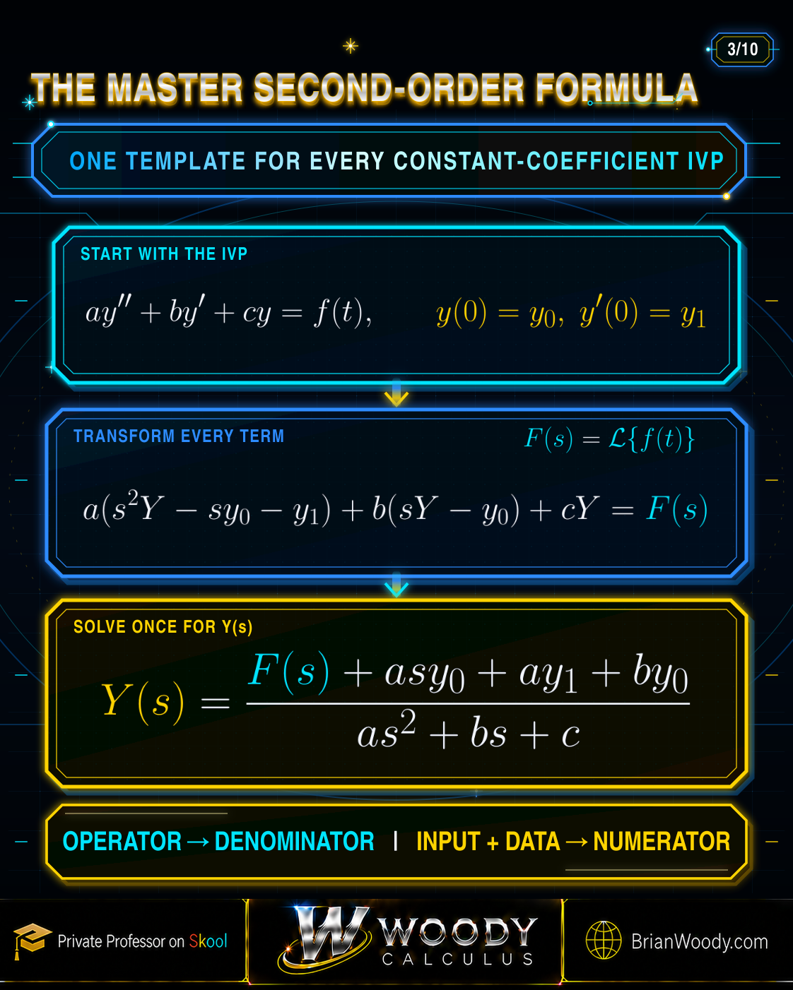
Transform
a y^{\prime\prime}+b y^{\prime}+cy=f(t),
\qquad y(0)=y_0,
\qquad y^{\prime}(0)=y_1.
\]
Using linearity and the derivative identities,
a(s^2Y-sy_0-y_1)+b(sY-y_0)+cY=F(s).
\]
Collect the \(Y\)-terms:
(as^2+bs+c)Y=F(s)+asy_0+ay_1+by_0.
\]
Division yields
\boxed{
Y(s)=\frac{F(s)+asy_0+ay_1+by_0}{as^2+bs+c}
}.
\]
How the characteristic equation reappears
The denominator \(as^2+bs+c\) is the characteristic polynomial with \(r\) replaced by \(s\). Its zeros are the poles of the transform. Those poles produce the same exponential modes found by the characteristic-equation method. Laplace transforms do not erase the underlying second-order theory; they package it with the forcing and initial data.
Part IV — The Seven-Step Method
Why the order of the steps matters
Students often know every transform rule but still lose the problem in the algebra. The usual causes are collecting \(Y(s)\) before substituting the initial values, leaving the denominator unfactored, or trying to invert a rational expression before it is decomposed.
The safest workflow is mechanical:
- Write \(Y(s)=\mathcal L\{y(t)\}\).
- Transform the equation without mental shortcuts.
- Replace \(y(0)\) and \(y^{\prime}(0)\) immediately.
- Move all non-\(Y\) terms to the other side.
- Factor the full coefficient of \(Y\).
- Make the expression invertible using partial fractions, shifting, completing the square, or convolution.
- Check the original problem, not merely the transformed equation.
What to write on an exam
A clean solution should show the derivative transforms, the substituted initial data, the isolated formula for \(Y(s)\), the decomposition, the inverse transform, and the verification. Skipping those transitions may save a few seconds, but it makes sign errors difficult to detect and partial credit difficult to earn.
Part V — Complete Worked IVP from Start to Finish
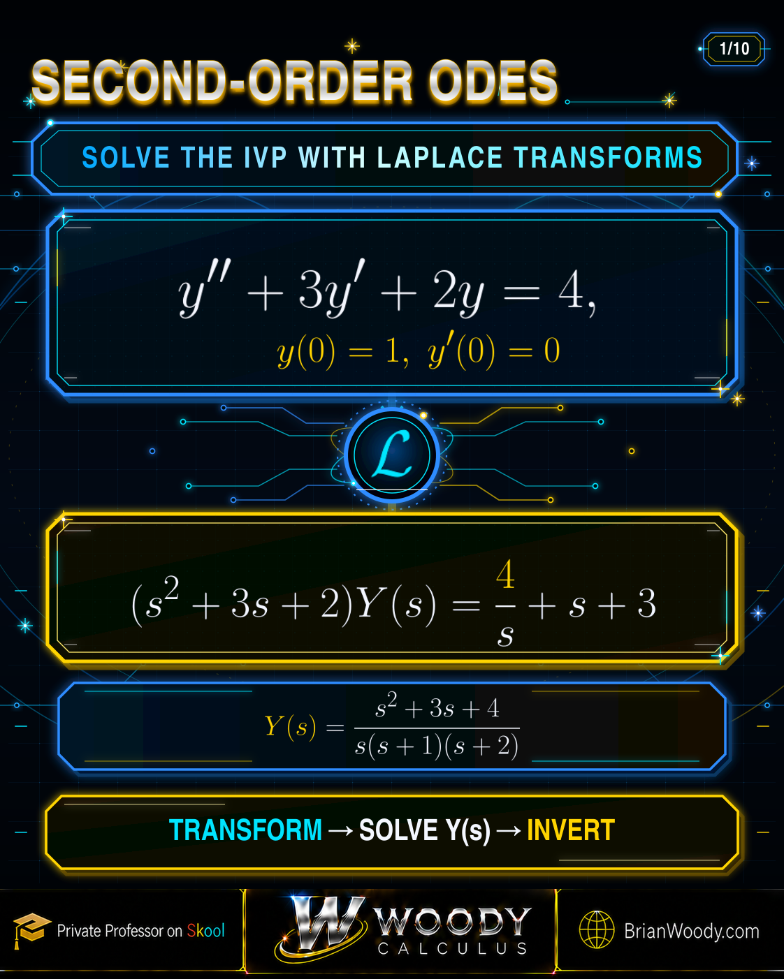
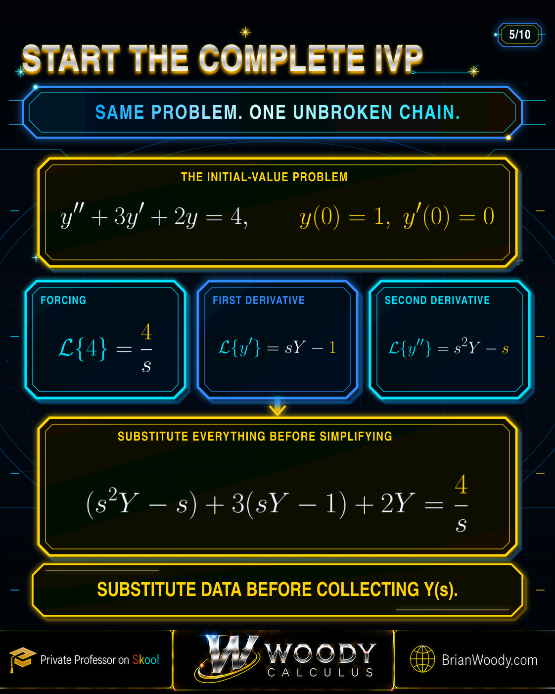
Solve
y^{\prime\prime}+3y^{\prime}+2y=4,
\qquad y(0)=1,
\qquad y^{\prime}(0)=0.
\]
Step 1: transform the equation
Let \(Y(s)=\mathcal L\{y(t)\}\). Then
\mathcal L\{4\}=\frac4s,
\qquad
\mathcal L\{y^{\prime}\}=sY-1,
\qquad
\mathcal L\{y^{\prime\prime}\}=s^2Y-s.
\]
Substitute every transformed piece:
(s^2Y-s)+3(sY-1)+2Y=\frac4s.
\]
Step 2: solve for \(Y(s)\)
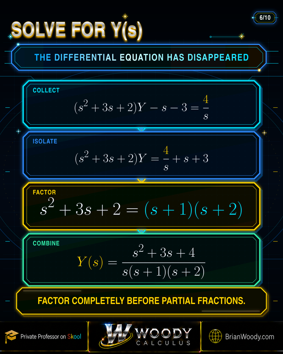
Collect the \(Y\)-terms:
(s^2+3s+2)Y-s-3=\frac4s.
\]
Isolate \(Y\) and factor:
Y=\frac{\frac4s+s+3}{(s+1)(s+2)}.
\]
Combine the numerator over the common denominator \(s\):
\boxed{
Y(s)=\frac{s^2+3s+4}{s(s+1)(s+2)}
}.
\]
Step 3: partial fractions
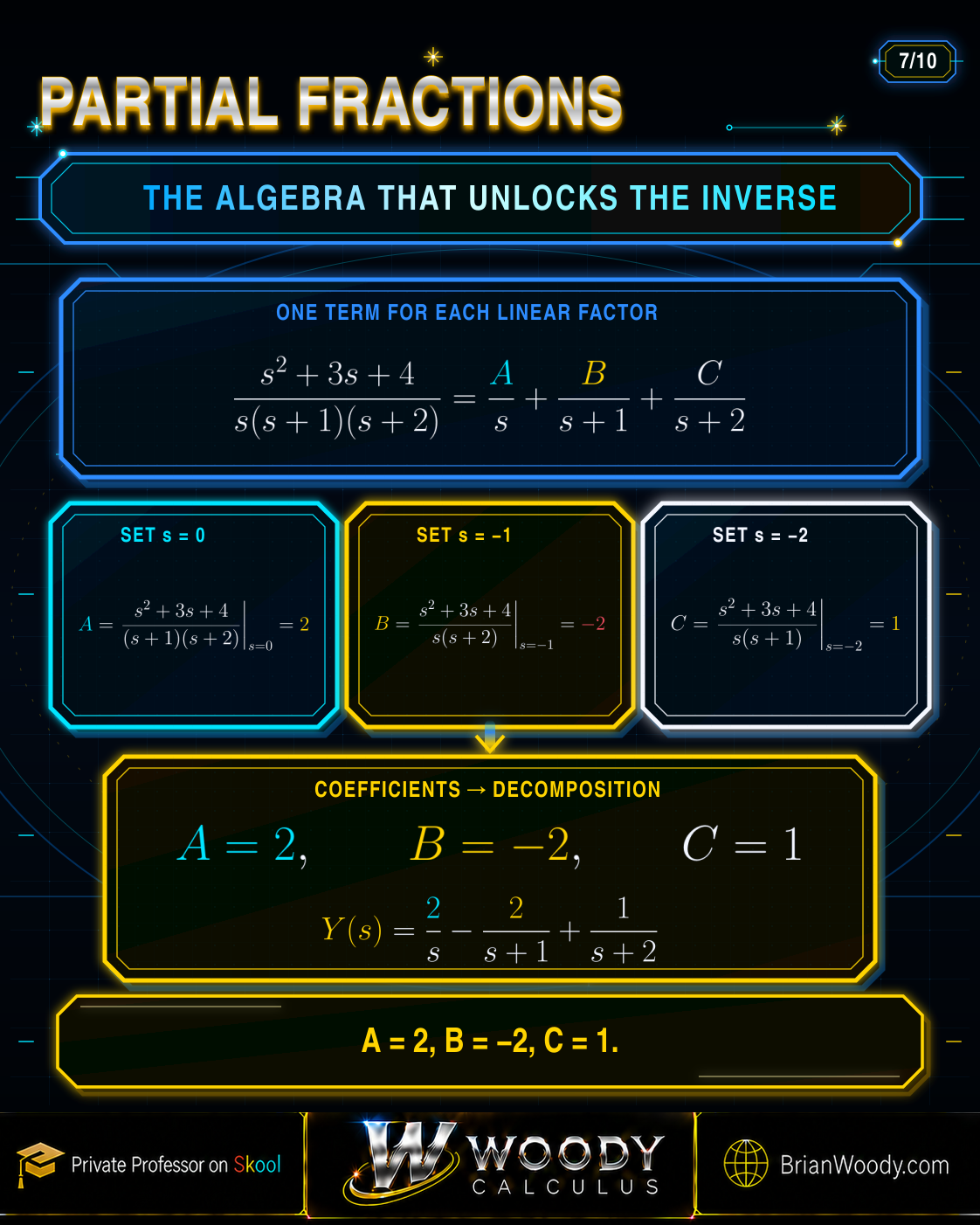
Write
\frac{s^2+3s+4}{s(s+1)(s+2)}
=\frac As+\frac B{s+1}+\frac C{s+2}.
\]
For distinct linear factors, cover each factor and substitute its zero:
A=\left.\frac{s^2+3s+4}{(s+1)(s+2)}\right|_{s=0}=2,
\]
B=\left.\frac{s^2+3s+4}{s(s+2)}\right|_{s=-1}=-2,
\]
C=\left.\frac{s^2+3s+4}{s(s+1)}\right|_{s=-2}=1.
\]
Therefore
Y(s)=\frac2s-\frac2{s+1}+\frac1{s+2}.
\]
Step 4: invert term by term
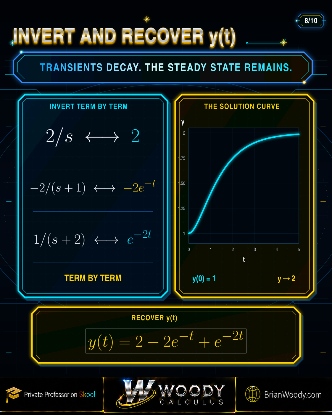
\mathcal L^{-1}\left\{\frac2s\right\}=2,
\qquad
\mathcal L^{-1}\left\{-\frac2{s+1}\right\}=-2e^{-t},
\qquad
\mathcal L^{-1}\left\{\frac1{s+2}\right\}=e^{-2t}.
\]
Hence
\boxed{y(t)=2-2e^{-t}+e^{-2t}}.
\]
The terms \(-2e^{-t}\) and \(e^{-2t}\) are transients. Both decay because their exponents are negative. The constant \(2\) is the steady-state response to the constant input \(4\).
Step 5: verify the IVP
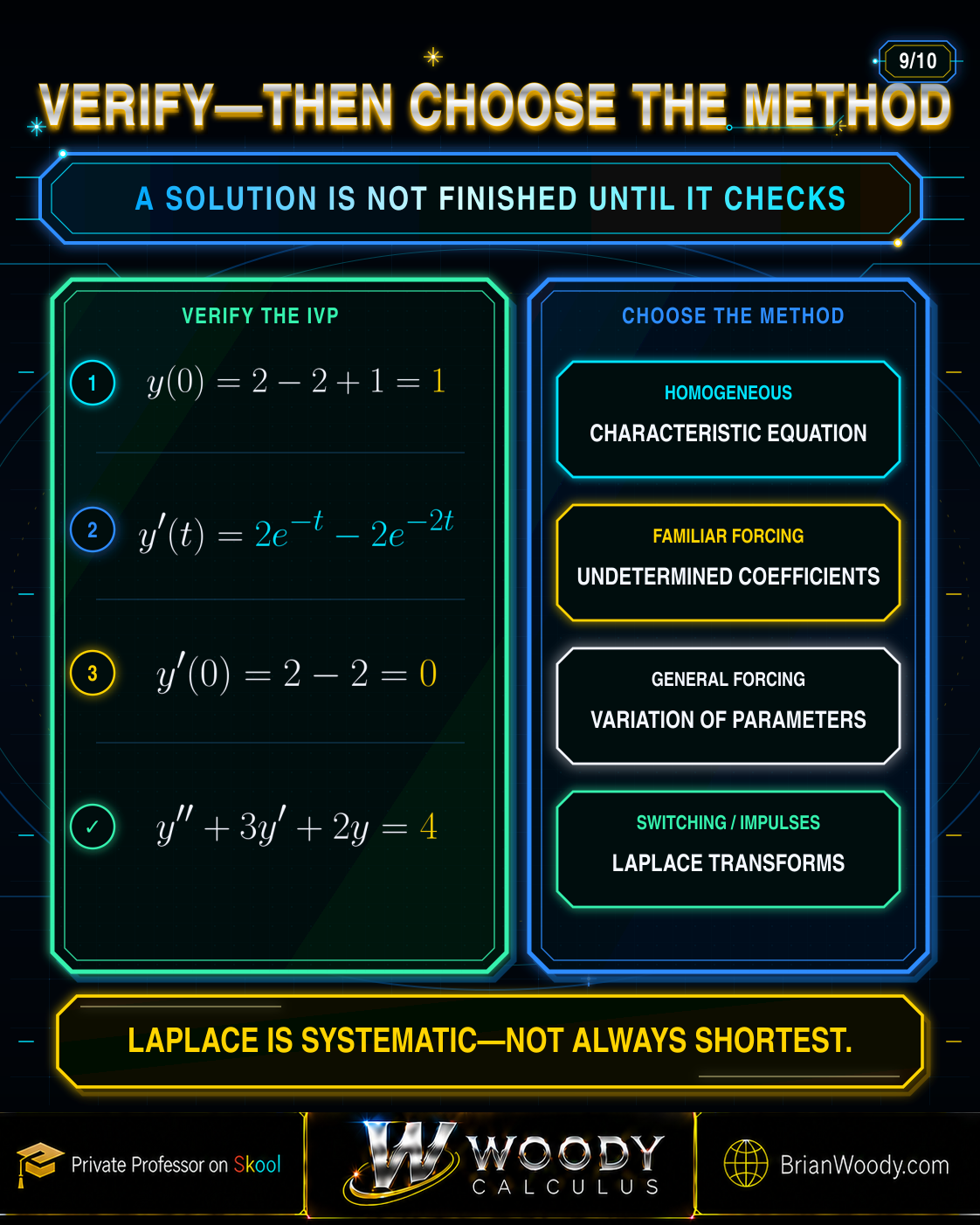
First check the initial values:
y(0)=2-2+1=1,
\]
y^{\prime}(t)=2e^{-t}-2e^{-2t},
\qquad
y^{\prime}(0)=2-2=0.
\]
Now compute
y^{\prime\prime}(t)=-2e^{-t}+4e^{-2t}.
\]
Substitution gives
\begin{aligned}
y^{\prime\prime}+3y^{\prime}+2y
&=(-2+6-4)e^{-t}+(4-6+2)e^{-2t}+4\\
&=4.
\end{aligned}
\]
Fast transform-domain checks
When their hypotheses are satisfied, the initial- and final-value theorems provide fast consistency checks:
y(0^+)=\lim_{s\to\infty}sY(s),
\qquad
\lim_{t\to\infty}y(t)=\lim_{s\to0}sY(s).
\]
For this example, the limits are \(1\) and \(2\). The final-value theorem requires the poles of \(sY(s)\) to lie in the open left half-plane. Do not use it when undamped oscillations or unstable poles prevent a finite final value.
Second complete example: resonant forcing
Consider
y^{\prime\prime}+y=\sin t,
\qquad y(0)=0,
\qquad y^{\prime}(0)=0.
\]
The forcing frequency equals the system’s natural frequency. Transforming gives
(s^2+1)Y(s)=\frac{1}{s^2+1},
\qquad
Y(s)=\frac{1}{(s^2+1)^2}.
\]
A standard inverse pair is
\mathcal L^{-1}\left\{\frac{1}{(s^2+1)^2}\right\}
=\frac12\bigl(\sin t-t\cos t\bigr).
\]
Therefore
\boxed{y(t)=\frac12\bigl(\sin t-t\cos t\bigr).}
\]
The factor \(t\) is the signature of resonance. In the transform domain, the forcing contributes another copy of \(s^2+1\), creating a repeated quadratic factor. In the time domain, the oscillation acquires a linearly growing envelope.
Verification is quick: \(y(0)=0\), \(y^{\prime}(0)=0\), and direct differentiation gives \(y^{\prime\prime}+y=\sin t\). This example shows why repeated factors matter even when the denominator has no real linear roots.
Part VI — Partial Fractions and Inverse-Transform Patterns
Solving for \(Y(s)\) is only the midpoint. The inverse transform becomes easy when the expression is rewritten as a sum of recognizable table entries. For rational transforms, that usually means factoring the denominator and using partial fractions.
Choose the decomposition from the denominator
| Denominator factor | Required numerator form | Typical inverse |
|---|---|---|
| Distinct linear factor \((s-a)\) | \(A/(s-a)\) | \(Ae^{at}\) |
| Repeated factor \((s-a)^m\) | \(A_1/(s-a)+\cdots+A_m/(s-a)^m\) | Exponentials multiplied by powers of \(t\) |
| Irreducible quadratic \((s-a)^2+b^2\) | \((B(s-a)+C)/((s-a)^2+b^2)\) | \(e^{at}\cos bt\) and \(e^{at}\sin bt\) |
| Improper rational function | Polynomial division first | Polynomial or impulse terms plus a proper fraction |
When the cover-up method works
The cover-up shortcut works directly for distinct linear factors. For
Y(s)=\frac{N(s)}{(s-r_1)(s-r_2)(s-r_3)},
\]
the coefficient of \(1/(s-r_1)\) is
A=\left.\frac{N(s)}{(s-r_2)(s-r_3)}\right|_{s=r_1}.
\]
Repeated roots and quadratic factors require the full template. The dependable order is: make the fraction proper, factor over the real numbers, write every required term, solve the coefficients, and only then invert.
Complete the square for oscillatory poles
If the denominator contains \(s^2+2\alpha s+\omega_0^2\), write it as
s^2+2\alpha s+\omega_0^2=(s+\alpha)^2+\bigl(\omega_0^2-\alpha^2\bigr).
\]
Then split the numerator into a multiple of \(s+\alpha\) plus a constant. That exposes shifted sine and cosine transform pairs and makes the damping factor \(e^{-\alpha t}\) visible.
Part VII — Unit Step Functions and Delayed Forcing
A unit step is an on-switch:
u(t-a)=
\begin{cases}
0,&t<a,\\
1,&t\ge a.
\end{cases}
\]
The exact value at the single point \(t=a\) does not affect its Laplace transform or ordinary differential-equation solution away from the switch. What matters is that the input is off before \(a\) and on after \(a\).
Rewrite a piecewise input before transforming
If an input changes from \(f_0(t)\) to \(f_1(t)\) at \(t=a\), write
f(t)=f_0(t)+u(t-a)\bigl[f_1(t)-f_0(t)\bigr].
\]
This says: begin with the old formula, then add exactly the correction needed when the switch turns on.
The second shifting theorem
The most useful delayed form is
\boxed{\mathcal L\{u(t-a)g(t-a)\}=e^{-as}G(s)}.
\]
Read it in both directions:
\boxed{\mathcal L^{-1}\{e^{-as}G(s)\}=u(t-a)g(t-a)}.
\]
The factor \(e^{-as}\) does not change the shape of \(g\). It delays the entire response by \(a\) units and keeps it zero beforehand.
Why the expression must use t minus a
The theorem requires a shifted function \(g(t-a)\), not merely \(u(t-a)g(t)\). If a piecewise formula contains \(u(t-a)q(t)\), introduce \(v=t-a\), rewrite \(q(t)=q(v+a)\), and then transform the resulting function of \(v\). This is the safest way to avoid a wrong exponential factor or a wrong time shift.
First shift versus second shift
| Rule | Transform statement | What changes in time? |
|---|---|---|
| First shifting theorem | \(F(s-a)\longleftrightarrow e^{at}f(t)\) | The function is multiplied by an exponential; it is not delayed. |
| Second shifting theorem | \(e^{-as}F(s)\longleftrightarrow u(t-a)f(t-a)\) | The whole function starts \(a\) units later. |
A shift inside \(F\), such as \(F(s-a)\), and a separate factor \(e^{-as}\) are different operations. Naming the theorem before using it prevents one of the most common transform-table errors.
Multiple switches fit in one formula
Suppose
f(t)=
\begin{cases}
0,&0\le t<2,\\
3,&2\le t<5,\\
0,&t\ge5.
\end{cases}
\]
Instead of solving three separate IVPs and matching constants, write
f(t)=3u(t-2)-3u(t-5).
\]
Its transform is
F(s)=\frac{3e^{-2s}}{s}-\frac{3e^{-5s}}{s}.
\]
Linearity then says the output is a delayed step response beginning at \(t=2\) minus an equal delayed step response beginning at \(t=5\). The system remembers the earlier input, so turning the force off does not generally make the output vanish instantly.
A finite pulse is two switches
A constant pulse of height \(M\) that begins at \(t=a\) and ends at \(t=b\) is
M\bigl[u(t-a)-u(t-b)\bigr],
\qquad 0<a<b,
\]
with transform
\frac{M}{s}\bigl(e^{-as}-e^{-bs}\bigr).
\]
The first step turns the input on; the second turns the same amount off.
Part VIII — Complete Example with a Switched Input
Solve the initially resting system
y^{\prime\prime}+3y^{\prime}+2y=u(t-1),
\qquad y(0)=0,
\qquad y^{\prime}(0)=0.
\]
1. Transform the equation
Because the initial values are zero, the derivative terms contribute no extra data:
(s^2+3s+2)Y(s)=\frac{e^{-s}}{s}.
\]
Therefore
Y(s)=e^{-s}\frac{1}{s(s+1)(s+2)}.
\]
2. Decompose the undelayed part
\frac{1}{s(s+1)(s+2)}
=\frac{1}{2s}-\frac{1}{s+1}+\frac{1}{2(s+2)}.
\]
Its inverse transform is
g(t)=\frac12-e^{-t}+\frac12e^{-2t}.
\]
3. Apply the delay
\boxed{
y(t)=u(t-1)\left[
\frac12-e^{-(t-1)}+\frac12e^{-2(t-1)}
\right].
}
\]
Equivalently,
y(t)=
\begin{cases}
0,&0\le t<1,\\
\dfrac12-e^{-(t-1)}+\dfrac12e^{-2(t-1)},&t\ge1.
\end{cases}
\]
4. Interpret and verify
The system does nothing before the input turns on. At the switching time, \(g(0)=0\) and \(g^{\prime}(0)=0\), so both \(y\) and \(y^{\prime}\) remain continuous. After the switch, the response approaches the constant steady state \(1/2\), consistent with setting derivatives to zero in \(2y=1\).
Part IX — Dirac Delta Impulses and Jump Behavior
The Dirac delta \(\delta(t-a)\) is not an ordinary finite-valued function. It is an idealized input concentrated at one instant and normalized so that
\int_{a-\varepsilon}^{a+\varepsilon}\delta(t-a)\,dt=1
\]
for every \(\varepsilon>0\). Its defining sampling property is
\int_0^{\infty}f(t)\delta(t-a)\,dt=f(a),
\qquad a>0,
\]
which immediately gives
\boxed{\mathcal L\{\delta(t-a)\}=e^{-as}}.
\]
Complete impulse-response example
Apply a unit impulse at \(t=1\) to the same initially resting system:
y^{\prime\prime}+3y^{\prime}+2y=\delta(t-1),
\qquad y(0)=0,
\qquad y^{\prime}(0)=0.
\]
Transforming gives
Y(s)=\frac{e^{-s}}{(s+1)(s+2)}
=e^{-s}\left(\frac{1}{s+1}-\frac{1}{s+2}\right).
\]
Therefore
\boxed{
y(t)=u(t-1)\left[e^{-(t-1)}-e^{-2(t-1)}\right].
}
\]
Why the derivative jumps
Integrate the differential equation across a small interval around \(t=1\). The integrals of \(3y^{\prime}\) and \(2y\) vanish in the limit when \(y\) stays bounded, while the impulse contributes 1. Thus
y^{\prime}(1^+)-y^{\prime}(1^-)=1.
\]
The displacement \(y\) remains continuous, but the velocity changes instantaneously. More generally, for
a y^{\prime\prime}+b y^{\prime}+cy=J\delta(t-t_0),
\]
the ordinary impulse jump is
y^{\prime}(t_0^+)-y^{\prime}(t_0^-)=\frac{J}{a},
\]
provided \(y\) itself remains continuous. This is the mathematical version of an instantaneous momentum kick in a mass-spring-damper model.
Step, finite pulse, and impulse are different inputs
| Input | Duration | Key quantity | Typical effect |
|---|---|---|---|
| Step \(u(t-a)\) | Persists after \(a\) | Height | Changes the sustained forcing and often the steady state |
| Finite pulse \(M[u(t-a)-u(t-b)]\) | From \(a\) to \(b\) | Height and duration | Forces the system temporarily |
| Impulse \(J\delta(t-a)\) | Idealized instant | Signed area \(J\) | Creates a state jump allowed by the differential order |
The distributional identity \(u^{\prime}(t-a)=\delta(t-a)\) explains why an impulse is the idealized derivative of an instantaneous switch. Correspondingly, integrating an impulse response produces a step response.
Which state variable can jump?
Integrating the ODE across the impulse is safer than memorizing a slogan. In a regular second-order equation with a delta on the right, \(y^{\prime}\) may jump while \(y\) stays continuous. A jump in \(y\) would make \(y^{\prime}\) contain a delta and \(y^{\prime\prime}\) contain a derivative of delta, which is not present in the stated forcing. Different equations or higher distributional inputs can produce different jump structures, so always use the differential equation itself.
Part X — Convolution and the Impulse-Response Formula
Convolution is the rule that combines an arbitrary input with a system’s response to one unit impulse. For causal functions \(f\) and \(g\),
(f*g)(t)=\int_0^t f(\tau)g(t-\tau)\,d\tau.
\]
The convolution theorem states
\boxed{\mathcal L\{f*g\}=F(s)G(s)}.
\]
The impulse response
For the zero-initial-condition equation
a y^{\prime\prime}+b y^{\prime}+cy=f(t),
\]
define the transfer function and impulse response by
H(s)=\frac{1}{as^2+bs+c},
\qquad
h(t)=\mathcal L^{-1}\{H(s)\}.
\]
Then \(Y=FH\), so
\boxed{y_{\mathrm{ZS}}(t)=(f*h)(t)
=\int_0^t f(\tau)h(t-\tau)\,d\tau.}
\]
Every infinitesimal piece of the input acts like a tiny delayed impulse. The integral adds all of those delayed impulse responses.
Convolution rebuilds the running example
For \(y^{\prime\prime}+3y^{\prime}+2y=f(t)\),
H(s)=\frac{1}{(s+1)(s+2)},
\qquad
h(t)=e^{-t}-e^{-2t}.
\]
With constant input \(f(t)=4\), the zero-state response is
\begin{aligned}
y_{\mathrm{ZS}}(t)
&=4\int_0^t\left[e^{-(t-\tau)}-e^{-2(t-\tau)}\right]d\tau\\
&=2-4e^{-t}+2e^{-2t}.
\end{aligned}
\]
The zero-input response determined by \(y(0)=1\) and \(y^{\prime}(0)=0\) is
y_{\mathrm{ZI}}(t)=2e^{-t}-e^{-2t}.
\]
Adding the two pieces gives
y(t)=y_{\mathrm{ZI}}+y_{\mathrm{ZS}}
=2-2e^{-t}+e^{-2t},
\]
exactly the solution obtained by direct inversion.
The convolution properties that simplify calculations
For causal functions for which the integrals exist, convolution is commutative, associative, and distributive:
f*g=g*f,
\qquad
(f*g)*q=f*(g*q),
\qquad
f*(g+q)=f*g+f*q.
\]
The identity element is the impulse:
f*\delta=f.
\]
A delayed impulse shifts a function:
f*\delta(t-a)=u(t-a)f(t-a).
\]
This is the convolution version of the second shifting theorem.
Green’s function and Duhamel’s principle
In this constant-coefficient causal setting, the impulse response \(h\) is also the causal Green’s function for the differential operator. The formula
y_{\mathrm{ZS}}(t)=\int_0^t h(t-\tau)f(\tau)\,d\tau
\]
is a form of Duhamel’s principle: build the response to an extended force by superposing responses to infinitesimal impulses. The vocabulary changes across differential equations, signals, physics, and engineering, but the mathematical object is the same.
Why the convolution integral stops at t
The upper limit is \(t\) because a causal system cannot respond at time \(t\) to an input applied later. Only values \(0\le\tau\le t\) contribute. If an input begins at \(a>0\), the integrand or the unit-step factor automatically removes all contributions before \(a\).
When convolution is the cleanest inverse
Use convolution when \(Y(s)\) is naturally a product \(F(s)H(s)\), the input transform is complicated, or you want a formula that works for an arbitrary forcing function. Partial fractions are usually shorter for a small rational expression. Convolution is more revealing when the system is fixed and the input changes.
Part XI — Transfer Functions, Poles, Transients, and Steady State
For a linear time-invariant system with zero initial conditions, the transfer function is the ratio of output transform to input transform:
\boxed{H(s)=\frac{Y(s)}{F(s)}=\frac{1}{as^2+bs+c}.}
\]
The zero-initial-condition requirement matters. Initial data create their own numerator terms, so the full ratio \(Y/F\) is not the transfer function when stored initial energy is present.
One function organizes three important responses
| Input | Transform | Output |
|---|---|---|
| Unit impulse \(\delta(t)\) | \(1\) | \(h(t)=\mathcal L^{-1}\{H(s)\}\) |
| Unit step \(u(t)\) | \(1/s\) | \(g(t)=\mathcal L^{-1}\{H(s)/s\}\) |
| Arbitrary causal input \(f(t)\) | \(F(s)\) | \((f*h)(t)\) |
The step response is the accumulated impulse response:
g(t)=\int_0^t h(\tau)\,d\tau,
\qquad
h(t)=g^{\prime}(t)
\]
where the derivative relation is interpreted appropriately at discontinuities.
Poles control the natural behavior
The poles are the zeros of \(as^2+bs+c\), after any legitimate cancellations have been considered. Their locations describe the homogeneous modes:
| Pole pattern | Time-domain mode | Behavior |
|---|---|---|
| Distinct negative real poles | \(C_1e^{r_1t}+C_2e^{r_2t}\) | Nonoscillatory decay |
| Repeated negative pole \(r\) | \((C_1+C_2t)e^{rt}\) | Critical-type decay |
| \(\alpha\pm i\beta\) | \(e^{\alpha t}(C_1\cos\beta t+C_2\sin\beta t)\) | Oscillation with envelope \(e^{\alpha t}\) |
| Any pole with positive real part | Growing exponential factor | Unstable natural response |
For a proper second-order transfer function with no hidden unstable modes, poles strictly in the open left half-plane give asymptotic decay of the impulse response. Poles on the imaginary axis require separate care because persistent oscillation may prevent a final value.
Transient versus steady-state response
The transient consists of modes that decay as time passes. The steady-state is what remains under a sustained input. In the running example,
y(t)=\underbrace{-2e^{-t}+e^{-2t}}_{\text{transient}}
+\underbrace{2}_{\text{steady state}}.
\]
The final-value theorem can find that constant without fully inverting:
\lim_{t\to\infty}y(t)=\lim_{s\to0}sY(s),
\]
but only when the poles of \(sY(s)\) are in the open left half-plane. Always check that hypothesis before using the shortcut.
Natural frequency and damping ratio
After dividing by the leading coefficient, a stable second-order denominator is often written
s^2+2\zeta\omega_n s+\omega_n^2,
\]
where \(\omega_n>0\) is the undamped natural frequency and \(\zeta\) is the damping ratio. The poles are
s=-\zeta\omega_n\pm\omega_n\sqrt{\zeta^2-1}.
\]
| Damping ratio | Pole type | Qualitative response |
|---|---|---|
| \(\zeta>1\) | Two negative real poles | Overdamped; no oscillation |
| \(\zeta=1\) | Repeated negative pole | Critically damped |
| \(0<\zeta<1\) | Complex poles with negative real part | Underdamped oscillation with decay |
| \(\zeta=0\) | Purely imaginary poles | Undamped persistent oscillation |
| \(\zeta<0\) | Poles with positive real part | Growing, unstable response |
This classification can be read before any inverse transform is performed. Laplace algebra gives the exact coefficients; pole geometry gives the qualitative story.
DC gain predicts the constant-input steady state
For a stable system and a constant input \(f(t)=K\), the transform is \(K/s\). When the final-value theorem applies,
y(\infty)=\lim_{s\to0}s\frac{K}{s}H(s)=K H(0).
\]
The number \(H(0)\) is the DC gain. In the running example, \(H(0)=1/2\), so a constant input of 4 produces steady value 2, while a unit step produces steady value \(1/2\).
A bridge to frequency response
Evaluating a stable transfer function along \(s=i\omega\) describes how the system changes the amplitude and phase of sinusoidal inputs. That is the bridge from an introductory Laplace-transform course to circuits, vibrations, signals, and control theory. The poles still matter: they encode the system’s natural frequencies and damping.
Part XII — Method Selection, Verification, and Common Mistakes
Laplace transforms are powerful because they are systematic, not because they are always shortest. Choose the method that matches the problem.
Which second-order method should you use?
| Problem type | Usually best first method | Why |
|---|---|---|
| Homogeneous constant-coefficient equation | Characteristic equation | Directly produces the natural modes |
| Polynomial, exponential, sine, or cosine forcing | Undetermined coefficients | Often shortest when the trial family is known |
| General continuous forcing | Variation of parameters or convolution | Works beyond the standard trial families |
| Initial-value problem with piecewise forcing | Laplace transforms and unit steps | Handles all intervals in one equation |
| Impulse forcing | Laplace transforms or jump conditions | Transforms delta inputs cleanly |
| Repeated use of the same linear system | Transfer function and impulse response | Separates the system from the input |
A verification checklist that catches most errors
- Initial data: Does the formula give the stated \(y(0)\) and \(y^{\prime}(0)\)?
- ODE: Does substitution reproduce the forcing on each open time interval?
- Switch timing: Is every delayed term multiplied by \(u(t-a)\) and written in terms of \(t-a\)?
- Continuity: For a finite step input, are \(y\) and \(y^{\prime}\) consistent across the switch for a regular second-order equation?
- Impulse jump: Does an impulse of area \(J\) create the required derivative jump \(J/a\)?
- Long-time behavior: Does the result agree with pole locations and any expected steady state?
- Transform check: If practical, transform the final answer and compare it with \(Y(s)\).
The twelve most common mistakes
1. Losing initial terms
\(\mathcal L\{y^{\prime\prime}\}\) is \(s^2Y-sy(0)-y^{\prime}(0)\), not just \(s^2Y\).
2. Using the wrong signs
Write the derivative formulas before inserting numbers.
3. Delaying substitution
Insert the initial values before collecting \(Y(s)\).
4. Forgetting the forcing transform
A constant \(K\) transforms to \(K/s\), not \(K\).
5. Inverting a product term by term
In general, \(\mathcal L^{-1}\{FG\}\ne fg\); it is \(f*g\).
6. Misreading \(e^{-as}\)
It means a delay: \(u(t-a)g(t-a)\), not \(e^{-at}g(t)\).
7. Omitting the step factor
A delayed formula must remain zero before its start time.
8. Incomplete partial fractions
Include every repeated power and a linear numerator over each irreducible quadratic.
9. Using the cover-up shortcut everywhere
It directly handles distinct linear factors, not every denominator pattern.
10. Treating delta as an ordinary function
Use its area, sampling rule, transform, or jump condition.
11. Defining \(H=Y/F\) with nonzero data
The transfer function is the zero-initial-condition input-output ratio.
12. Using final value without checking poles
The theorem has stability hypotheses; it is not a universal limit shortcut.
What if the initial time is not zero?
If the data are given at \(t=t_0\), introduce the shifted time \(\tau=t-t_0\) and define \(z(\tau)=y(\tau+t_0)\). Then \(z(0)=y(t_0)\) and \(z^{\prime}(0)=y^{\prime}(t_0)\), so the standard one-sided formulas apply. Remember to rewrite the forcing in terms of \(\tau\) and translate the final answer back to \(t\).
Limits of the simple Laplace workflow
- Nonlinear equations: the transform of a product such as \(y^2\) or \(yy^{\prime}\) does not reduce to a simple product of transforms.
- Variable coefficients: terms such as \(ty^{\prime\prime}\) introduce derivatives of \(Y(s)\), so the transformed problem may still be a differential equation.
- Unknown transform or difficult inversion: a formal expression for \(Y(s)\) may be less useful than a numerical method or a convolution integral.
- Boundary-value problems: the one-sided transform is tailored to data at one initial time, not conditions split across two endpoints.
These are method-selection limits, not failures of the theory. Knowing when Laplace transforms simplify a problem is part of mastering them.
Part XIII — Mastery Map and Practice Set
The complete concept chain
Ten mastery problems
- Derive \(\mathcal L\{y^{\prime\prime}\}\) from the first-derivative formula.
- Solve \(y^{\prime\prime}+5y^{\prime}+6y=0\), \(y(0)=2\), \(y^{\prime}(0)=-1\), using Laplace transforms.
- Solve \(y^{\prime\prime}+y=\sin t\), \(y(0)=0\), \(y^{\prime}(0)=0\).
- Rewrite the input that equals 0 for \(t<2\), 3 for \(2\le t<5\), and 0 for \(t\ge5\) using unit steps.
- Find the transform of \(u(t-2)(t-2)^2\).
- Solve \(y^{\prime\prime}+3y^{\prime}+2y=u(t-2)\) with zero initial data.
- Find the impulse response of \(y^{\prime\prime}+4y^{\prime}+4y=f(t)\).
- For \(2y^{\prime\prime}+y=6\delta(t-3)\), determine the jump in \(y^{\prime}\) at \(t=3\).
- Write the zero-state solution of \(y^{\prime\prime}+3y^{\prime}+2y=f(t)\) as a convolution integral.
- Explain why the final-value theorem fails for \(Y(s)=1/(s^2+1)\).
Open the concise answer key
- \(s(sY-y(0))-y^{\prime}(0)=s^2Y-sy(0)-y^{\prime}(0)\).
- \(y(t)=5e^{-2t}-3e^{-3t}\).
- \(y(t)=\tfrac12(\sin t-t\cos t)\).
- \(3[u(t-2)-u(t-5)]\).
- \(2e^{-2s}/s^3\).
- \(u(t-2)[\tfrac12-e^{-(t-2)}+\tfrac12e^{-2(t-2)}]\).
- \(h(t)=te^{-2t}\).
- \(y^{\prime}(3^+)-y^{\prime}(3^-)=6/2=3\).
- \(y(t)=\int_0^t f(\tau)[e^{-(t-\tau)}-e^{-2(t-\tau)}]d\tau\).
- The poles of \(sY(s)=s/(s^2+1)\) lie at \(s=\pm i\), not in the open left half-plane; the time response does not approach a finite limit.
Woody mastery check
You understand this chapter when you can reconstruct the derivative formulas, derive the master formula, execute the seven-step chain, translate a piecewise input into steps, interpret \(e^{-as}\), explain the delta jump, and derive \(y_{\mathrm{ZS}}=f*h\) from \(Y=FH\) without looking.
References and Further Study
This lesson’s notation and core transform identities align with standard undergraduate differential-equations treatments. For additional worked explanations, consult the following open educational resources:
- Ohio State Ximera: Introduction to the Laplace Transform
- Ohio State Ximera: Solving Initial-Value Problems with Laplace Transforms
- Ohio State Ximera: The Unit Step Function
- Ohio State Ximera: Constant-Coefficient Equations with Impulses
- Ohio State Ximera: Convolution
- Woody Calculus: Laplace Transforms Help
- Woody Calculus: Laplace Transforms as Differential-Equation Algebra
Frequently Asked Questions
What does the Laplace transform do to a second-order differential equation?
It converts differentiation in time into algebra in s. The differential operator becomes a polynomial multiplying Y(s), while the initial values appear explicitly in the numerator.
What is the Laplace transform of y double prime?
If Y(s) is the Laplace transform of y(t), then the transform of y double prime is s²Y(s) − sy(0) − y prime(0).
Why do initial conditions appear automatically in the Laplace method?
They arise from integration by parts in the derivative formulas. A second derivative records both y(0) and y prime(0), which is why the transformed algebra already contains the IVP data.
What is the master formula for a second-order constant-coefficient IVP?
For ay double prime + by prime + cy = f(t), with y(0) = y₀ and y prime(0) = y₁, Y(s) = [F(s) + asy₀ + ay₁ + by₀] divided by [as² + bs + c].
When should I use Laplace transforms instead of the characteristic equation?
Use the characteristic equation first for a homogeneous constant-coefficient ODE. Laplace transforms are especially useful when initial conditions, piecewise inputs, delayed switching, or impulses are central to the problem.
What is the Laplace transform of a constant K?
The transform is K/s, not K. Forgetting the factor 1/s is a common source of errors in forced differential equations.
Why are partial fractions used in inverse Laplace transforms?
They rewrite a rational function as a sum of standard transform pairs. Each simpler term can then be inverted separately.
When does the Heaviside cover-up method work?
It works directly for coefficients attached to distinct linear factors. Repeated factors and irreducible quadratics require the complete partial-fraction template.
What happens when the Laplace denominator has a repeated root?
The decomposition must include every power of the repeated factor. In the time domain, repeated poles produce powers of t multiplying an exponential, such as te to the rt.
What is the unit step function?
The unit step u(t − a) is 0 before t = a and 1 after t = a. It models an input or correction that turns on at a specified time.
What is the difference between the first and second shifting theorems?
The first shifting theorem moves s and corresponds to multiplying by an exponential in time. The second shifting theorem multiplies by e to the negative as and corresponds to delaying a time-domain function until t = a.
How do I rewrite a piecewise forcing function with unit steps?
Start with the first formula and add u(t − a) times the change from the old formula to the new formula at each switching time.
What does the factor e to the negative as mean in a Laplace transform?
It means a time delay of a units. The inverse is u(t − a)g(t − a), so the response is zero before t = a and then follows the original shape.
How do I represent a finite rectangular pulse?
A pulse of height M from t = a to t = b is M[u(t − a) − u(t − b)]. The first step turns it on and the second turns it off.
What is the Dirac delta function?
It is an idealized impulse concentrated at one instant with a specified total area. It is handled through its sampling property, transform, or jump conditions rather than as an ordinary finite-valued function.
What is the Laplace transform of delta of t minus a?
The Laplace transform of δ(t − a) is e to the negative as for a greater than or equal to zero.
What jumps when a second-order ODE receives an impulse?
For ay double prime + by prime + cy = Jδ(t − t₀), an ordinary impulse keeps y continuous and changes y prime by J/a, under the usual regularity assumptions.
What is an impulse response?
The impulse response h(t) is the zero-initial-condition output produced by a unit impulse. For ay double prime + by prime + cy = f(t), it is the inverse Laplace transform of 1 divided by as² + bs + c.
What is a transfer function?
For zero initial conditions, the transfer function is H(s) = Y(s)/F(s). It separates the fixed system from the input and encodes the poles and natural response.
Why must a transfer function use zero initial conditions?
Nonzero initial data add independent numerator terms that are not caused by F(s). Setting the initial state to zero isolates the input-output behavior of the system.
What is convolution in Laplace transforms?
Convolution is (f ∗ h)(t) = the integral from 0 to t of f(τ)h(t − τ)dτ. Its Laplace transform is the product F(s)H(s).
Is the inverse Laplace transform of F(s)G(s) equal to f(t)g(t)?
No. In general, the inverse transform of a product is the convolution f ∗ g, not the pointwise product fg.
How are the step response and impulse response related?
For a causal system, the unit-step response is the integral of the impulse response. Away from discontinuities, the impulse response is the derivative of the step response.
What are zero-input and zero-state responses?
The zero-input response comes from the initial conditions with external forcing set to zero. The zero-state response comes from the forcing with initial conditions set to zero. Their sum is the complete response.
What do the poles of Y(s) or H(s) tell us?
They determine the natural exponential or oscillatory modes. Their locations indicate decay, persistent oscillation, or growth and therefore reveal transient behavior and stability.
When is a second-order system asymptotically stable?
For a standard continuous-time second-order system with no hidden unstable modes, asymptotic stability requires both poles to have negative real parts.
When can I use the final-value theorem?
Use it only when the poles of sY(s) lie in the open left half-plane. Unstable poles or persistent imaginary-axis oscillations invalidate the shortcut.
What does the initial-value theorem say?
When its regularity conditions hold, y(0 plus) equals the limit of sY(s) as s approaches infinity. It is a fast consistency check, not a replacement for the full initial conditions.
Can Laplace transforms solve variable-coefficient differential equations?
Sometimes, but not usually with the simple algebraic workflow in this lesson. Multiplication by t becomes differentiation with respect to s, and many variable-coefficient equations are better handled by series or other methods.
How should I verify a Laplace-transform solution?
Check every initial condition, substitute into the ODE on each open time interval, verify switch or impulse behavior, and compare the long-time response with the pole structure and expected steady state.
Keep Building Your Differential Equations Map
Laplace transforms become much easier when the equation, the input, and the system response are treated as one connected structure. Continue with the characteristic-equation guide, the phase portraits lesson, or the complete Woody Calculus Math Library. For guided practice and direct help, join the Woody Calculus Mastery Lab.