Error bounds are one of the most important ideas in Calculus 2 and AP Calculus BC.
Error bounds are critical in numerical analysis, engineering, physics, computer science, and applied mathematics because they transform an approximation from a guess into a guaranteed range of accuracy.
Students often learn how to approximate a number or a function. But the deeper question is:
How accurate is the approximation?
That question is what error bounds answer.
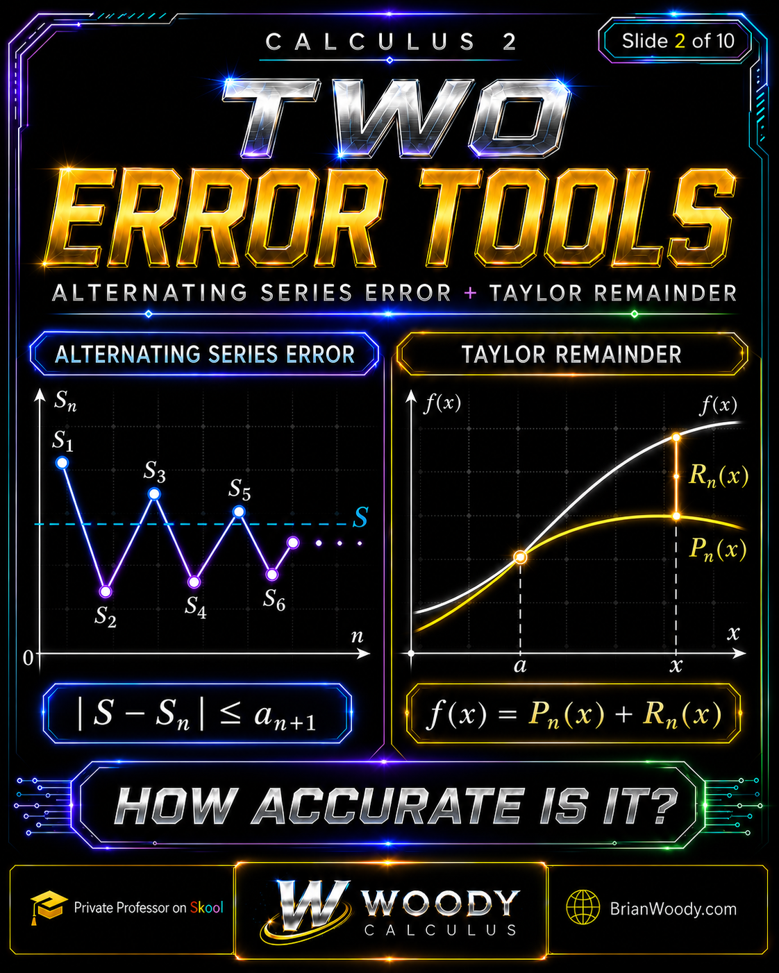
In Calculus 2, two of the biggest error-control tools are:
- Alternating series error: controls the error when an alternating series is approximated by a partial sum.
- Taylor remainder: controls the error when a function is approximated by a Taylor polynomial.
The central idea is simple:
\text{exact value}=\text{approximation}+\text{error}.
\]
For Taylor polynomials, this becomes:
f(x)=P_n(x)+R_n(x).
\]
For alternating series, this becomes:
S=S_n+R_n.
\]
This Woody Calculus lesson explains both tools, shows when to use each one, and gives complete worked examples for the alternating series for \(\ln 2\) and the Taylor approximation for \(\sin x\).
Estimated read time: 14–18 minutes.
Last updated: .
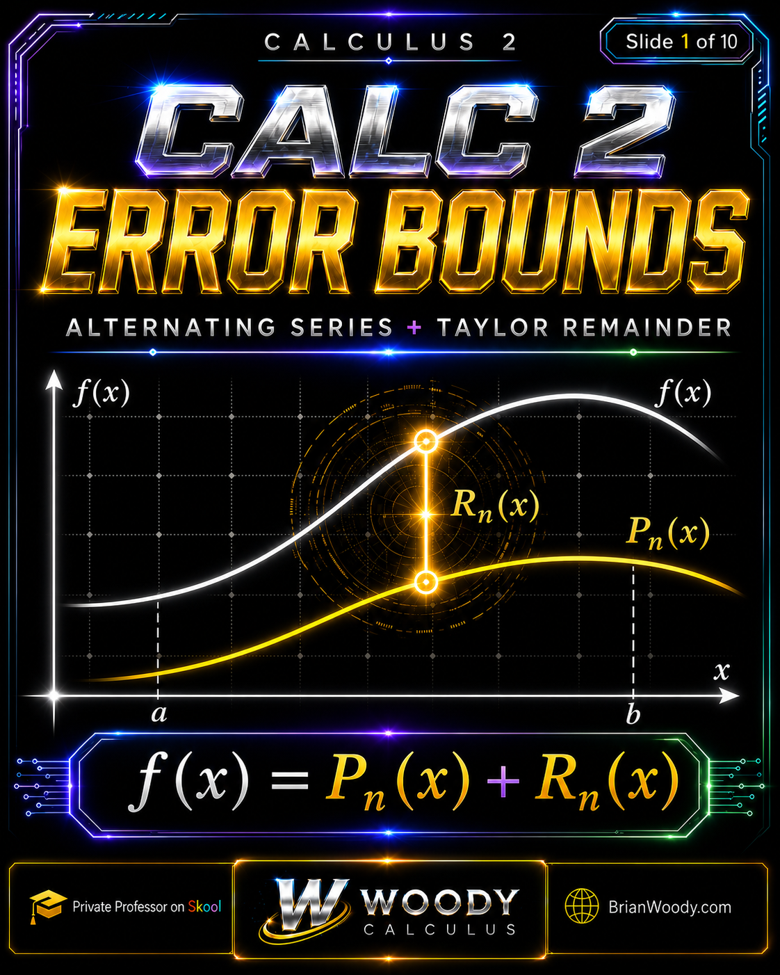
What Are Error Bounds?
An error bound is a guarantee on how far an approximation can be from the exact value.
If \(A\) is the exact value and \(A_n\) is an approximation, then the error is:
\text{error}=A-A_n.
\]
Usually, we care about the size of the error:
\left|A-A_n\right|.
\]
An error bound gives a number that the error cannot exceed:
\left|A-A_n\right|\le \text{bound}.
\]
That is powerful because it lets us say things like:
This approximation is guaranteed to be within \(0.001\) of the true value.
In Calculus 2, this matters because students often use partial sums or Taylor polynomials instead of exact values.
Two Error Tools in Calculus 2
There are two major error-bound tools students see in Calculus 2 and AP Calculus BC.
| Error Tool | Used For | Main Formula | Main Idea |
|---|---|---|---|
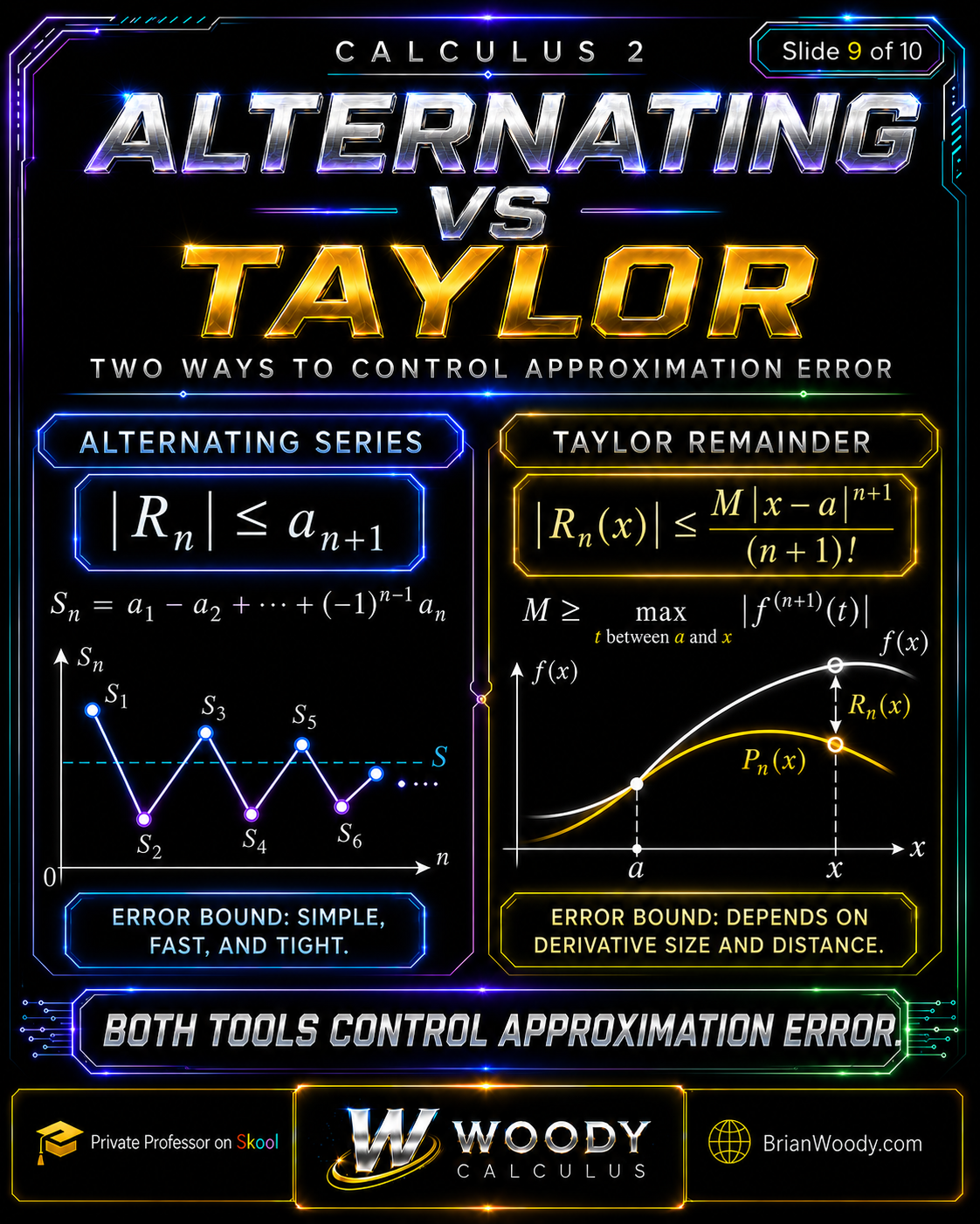
| Alternating Series Error | Alternating series partial sums | \(\left|S-S_n\right|\le a_{n+1}\) | The error is no bigger than the first term left out. |
| Taylor Remainder / Lagrange Error Bound | Taylor polynomial approximations | \(\left|R_n(x)\right|\le \frac{M|x-a|^{n+1}}{(n+1)!}\) | The error depends on derivative size and distance from the center. |
Both tools answer the same question:
How accurate is it?
Alternating Series Error
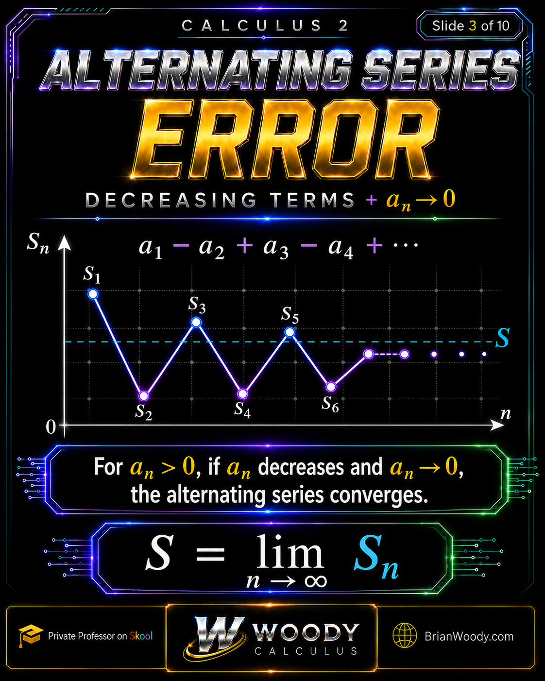
An alternating series has terms that switch signs:
a_1-a_2+a_3-a_4+\cdots.
\]
Here the numbers \(a_n\) are positive.
The alternating series test says that if:
- \(a_n>0\),
- \(a_n\) decreases,
- \(\lim_{n\to\infty}a_n=0\),
then the alternating series converges.
In symbols:
S=\lim_{n\to\infty}S_n.
\]
The partial sums bounce above and below the true sum, getting closer as the terms shrink.
That bouncing is exactly why the error can be controlled so cleanly.
The First Omitted Term Rule
The alternating series error bound is one of the cleanest formulas in Calculus 2:
\boxed{
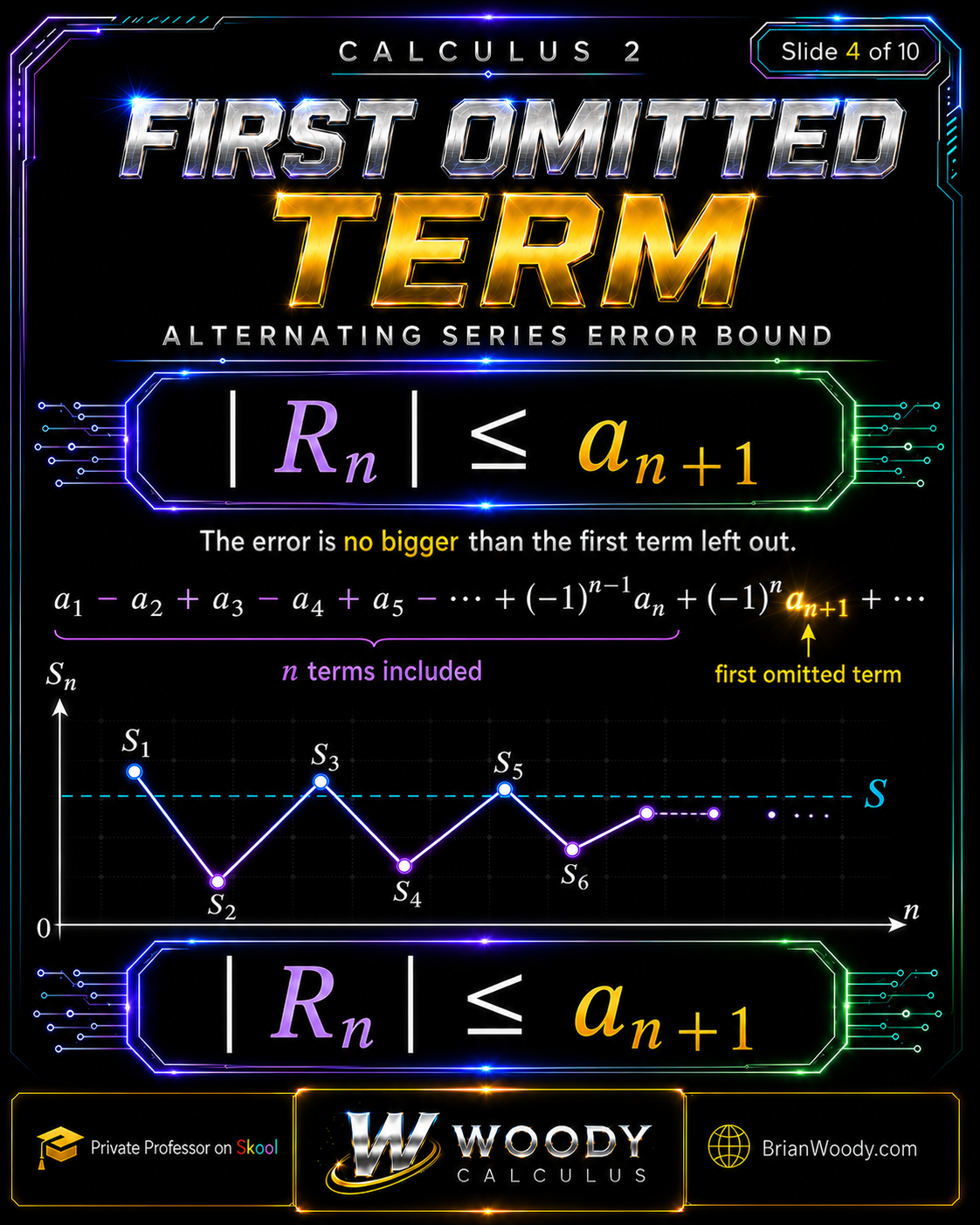
\left|S-S_n\right|\le a_{n+1}.
}
\]
Since \(R_n=S-S_n\), we can also write:
\boxed{
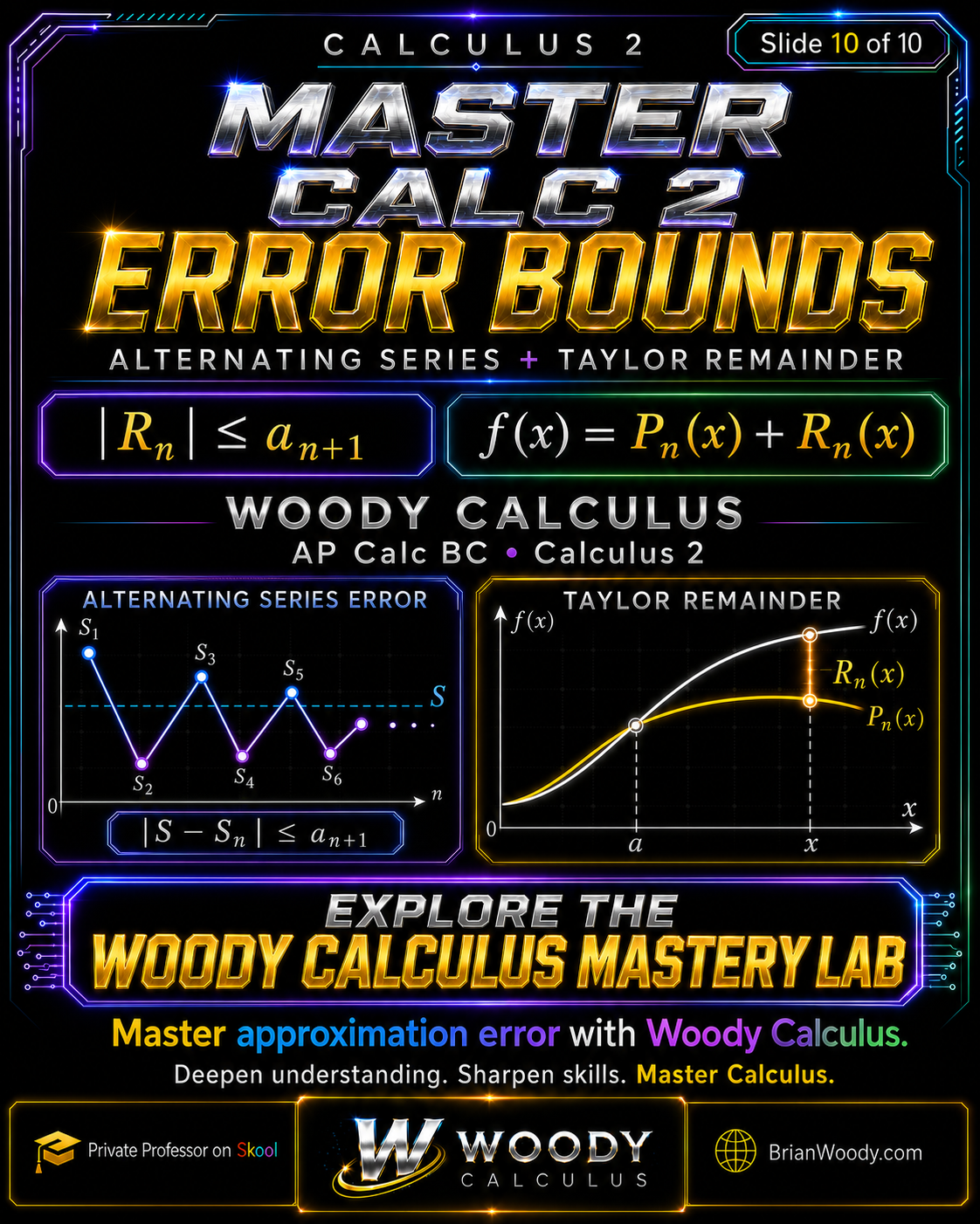
\left|R_n\right|\le a_{n+1}.
}
\]
This means:
The error is no bigger than the first term left out.
That phrase matters. If you use \(n\) terms, then the first omitted term is the \((n+1)\)-st term.
For an alternating series:
S_n=a_1-a_2+a_3-a_4+\cdots+(-1)^{n-1}a_n.
\]
The next term has size \(a_{n+1}\), so:
\left|S-S_n\right|\le a_{n+1}.
\]
Alternating Series Error Example: \(\ln 2\)
A classic alternating series is:
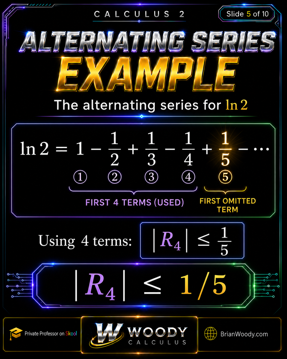
\ln 2=1-\frac12+\frac13-\frac14+\frac15-\cdots.
\]
Suppose we approximate \(\ln 2\) using the first four terms:
S_4=1-\frac12+\frac13-\frac14.
\]
Compute:
S_4=\frac{12}{12}-\frac{6}{12}+\frac{4}{12}-\frac{3}{12}
=\frac{7}{12}.
\]
The first omitted term is:
\frac15.
\]
So the alternating series error bound gives:
\boxed{
\left|R_4\right|\le \frac15.
}
\]
Plain-language answer: if we approximate \(\ln 2\) by the first four terms of its alternating series, then the error is no bigger than \(1/5\).
This bound is easy to compute, but not always tight. The true error is smaller than the bound. The point is that the bound gives a guaranteed maximum error.
Taylor Polynomial Error
Now switch from approximating a number with a partial sum to approximating a function with a polynomial.
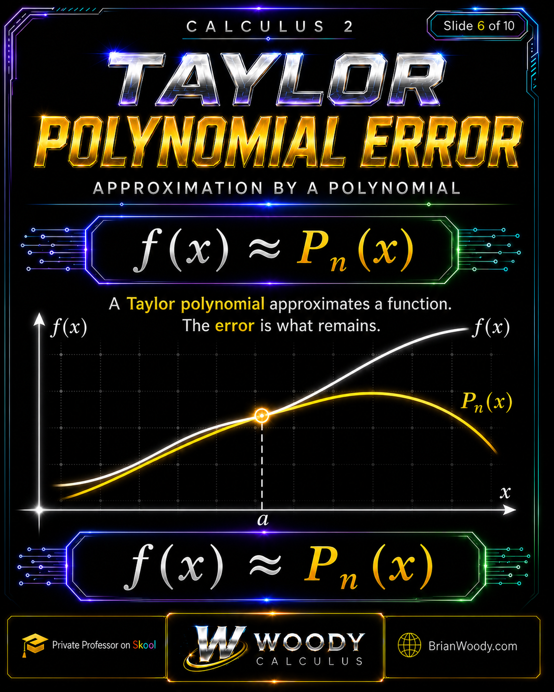
A Taylor polynomial \(P_n(x)\) approximates a function \(f(x)\) near a center \(a\):
f(x)\approx P_n(x).
\]
But approximation is not equality. The difference between the function and the Taylor polynomial is the error:
R_n(x)=f(x)-P_n(x).
\]
So the exact relationship is:
\boxed{
f(x)=P_n(x)+R_n(x).
}
\]
Here:
- \(f(x)\) is the true function value,
- \(P_n(x)\) is the Taylor polynomial approximation,
- \(R_n(x)\) is the Taylor remainder, or error.
Taylor Remainder and Lagrange Error Bound
The Taylor remainder bound tells us how large \(R_n(x)\) can be.
This formula is also called the Lagrange error bound or Lagrange remainder. This is the name many AP Calculus BC students see when learning how to bound Taylor polynomial error.
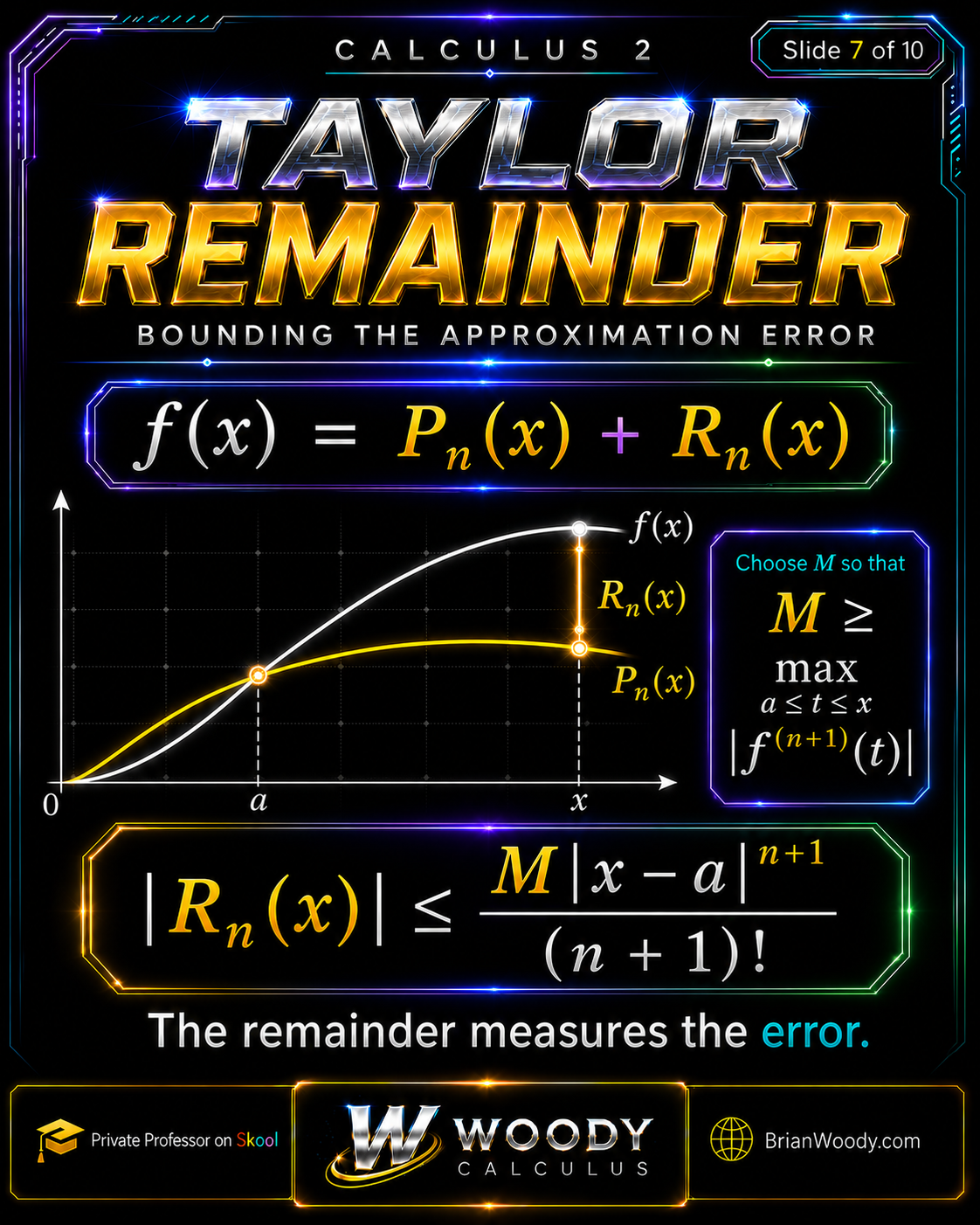
If \(P_n(x)\) is the \(n\)-th Taylor polynomial for \(f(x)\) centered at \(a\), then:
\boxed{
\left|R_n(x)\right|
\le
\frac{M|x-a|^{n+1}}{(n+1)!}.
}
\]
Here \(M\) must satisfy:
M\ge \max \left|f^{(n+1)}(t)\right|
\]
on the interval between \(a\) and \(x\). More precisely:
M\ge \max_{\min(a,x)\le t\le \max(a,x)}
\left|f^{(n+1)}(t)\right|.
\]
\(M\) is the maximum size of the \((n+1)\)-st derivative on the interval between the center and your point, not just the derivative value at the center or at one convenient point.
This formula has three ingredients:
- Derivative size: controlled by \(M\).
- Distance from the center: controlled by \(|x-a|^{n+1}\).
- Polynomial degree: controlled by \((n+1)!\).
Taylor error gets smaller when \(x\) is close to \(a\), when the derivatives are not too large, and when a higher-degree Taylor polynomial is used.
Taylor Remainder Example: Approximating \(\sin(0.3)\)
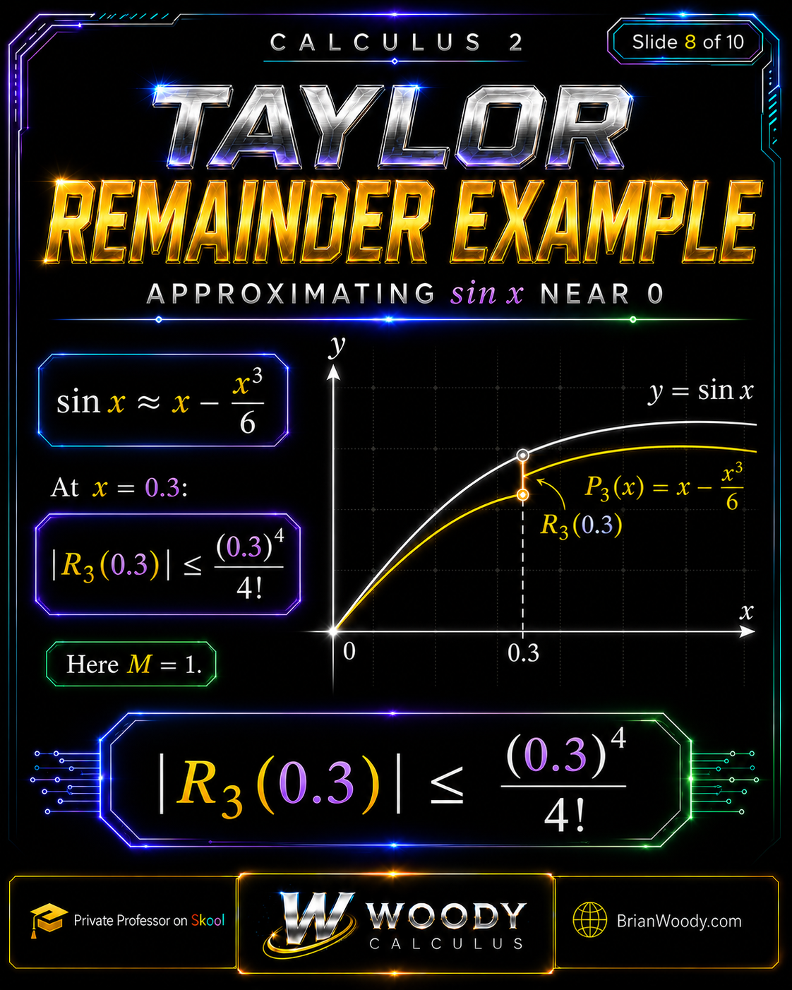
Now approximate \(\sin x\) near \(0\) using the third-degree Maclaurin polynomial:
\sin x\approx x-\frac{x^3}{6}.
\]
So:
P_3(x)=x-\frac{x^3}{6}.
\]
At \(x=0.3\):
P_3(0.3)=0.3-\frac{(0.3)^3}{6}.
\]
Since:
(0.3)^3=0.027,
\]
we get:
P_3(0.3)=0.3-\frac{0.027}{6}=0.3-0.0045=0.2955.
\]
Now bound the error.
For \(P_3\), the Taylor remainder uses the fourth derivative. Since:
f(x)=\sin x,
\]
we have:
f^{(4)}(x)=\sin x.
\]
A simple safe bound is:
M=1,
\]
because:
|\sin t|\le 1
\]
for all \(t\).
The Lagrange error bound gives:
\left|R_3(0.3)\right|
\le
\frac{1\cdot |0.3-0|^4}{4!}.
\]
So:
\boxed{
\left|R_3(0.3)\right|\le \frac{(0.3)^4}{4!}.
}
\]
Since \((0.3)^4=0.0081\) and \(4!=24\):
\left|R_3(0.3)\right|
\le
\frac{0.0081}{24}
=
0.0003375.
\]
Plain-language answer: using \(x-\frac{x^3}{6}\) to approximate \(\sin(0.3)\), the error is at most \(0.0003375\).
\sin(0.3)\approx 0.2955
\quad\text{with error at most}\quad
0.0003375.
\]
Alternating Series Error vs Taylor Remainder
Alternating series error and Taylor remainder both control approximation error, but they are used in different situations.
| Question | Alternating Series Error | Taylor Remainder / Lagrange Error Bound |
|---|---|---|
| What are you approximating? | A series sum \(S\) | A function value \(f(x)\) |
| What is the approximation? | A partial sum \(S_n\) | A Taylor polynomial \(P_n(x)\) |
| What is the error? | \(R_n=S-S_n\) | \(R_n(x)=f(x)-P_n(x)\) |
| Main bound | \(\left|R_n\right|\le a_{n+1}\) | \(\left|R_n(x)\right|\le \frac{M|x-a|^{n+1}}{(n+1)!}\) |
| What makes it easy? | The first omitted term | A manageable bound on a higher derivative |
The alternating series bound is usually faster. The Taylor remainder bound is more flexible.
The Woody Calculus summary is:
Alternating series error uses the next term. Taylor remainder uses derivative size and distance from the center.
Complete Worked Summary
Alternating Series Error Summary
Suppose:
S=a_1-a_2+a_3-a_4+\cdots,
\]
where \(a_n>0\), \(a_n\) decreases, and \(a_n\to0\).
Then:
S=\lim_{n\to\infty}S_n.
\]
If \(S_n\) uses the first \(n\) terms, then:
\boxed{
\left|S-S_n\right|\le a_{n+1}.
}
\]
For:
\ln2=1-\frac12+\frac13-\frac14+\frac15-\cdots,
\]
using four terms gives:
S_4=\frac{7}{12}
\]
and:
\boxed{
\left|R_4\right|\le \frac15.
}
\]
Taylor Remainder / Lagrange Error Bound Summary
If:
f(x)=P_n(x)+R_n(x),
\]
then:
R_n(x)=f(x)-P_n(x).
\]
If \(M\) bounds \(\left|f^{(n+1)}(t)\right|\) between \(a\) and \(x\), then:
\boxed{
\left|R_n(x)\right|
\le
\frac{M|x-a|^{n+1}}{(n+1)!}.
}
\]
For:
\sin x\approx x-\frac{x^3}{6}
\]
at \(x=0.3\), using \(M=1\):
\boxed{
\left|R_3(0.3)\right|
\le
\frac{(0.3)^4}{4!}
=
0.0003375.
}
\]
Common Mistakes
Mistake 1: Using the alternating series error bound when the series is not alternating
The formula \(\left|S-S_n\right|\le a_{n+1}\) requires an alternating series with positive terms \(a_n\) that decrease to zero.
Mistake 2: Forgetting the first omitted term
If you use \(n\) terms, the error bound uses \(a_{n+1}\), not \(a_n\).
Mistake 3: Treating Taylor approximation as exact equality
A Taylor polynomial is an approximation:
f(x)\approx P_n(x).
\]
The exact statement is:
f(x)=P_n(x)+R_n(x).
\]
Mistake 4: Choosing \(M\) incorrectly
For Taylor remainder, \(M\) must bound the absolute value of the \((n+1)\)-st derivative on the interval between the center \(a\) and the input \(x\).
Mistake 5: Forgetting the factorial
The Taylor remainder bound includes \((n+1)!\) in the denominator:
\left|R_n(x)\right|
\le
\frac{M|x-a|^{n+1}}{(n+1)!}.
\]
The Woody Calculus Error Bounds Checklist
The Woody Calculus Method for Error Bounds
The Woody Calculus method is to identify the approximation type first, then choose the correct error tool.
- Ask what is being approximated: a series sum or a function value?
- If it is an alternating series, check the conditions: \(a_n>0\), decreasing, and \(a_n\to0\).
- For alternating series error, find the first omitted term: \(a_{n+1}\).
- If it is a Taylor polynomial, identify the center \(a\), degree \(n\), and input \(x\).
- Find the \((n+1)\)-st derivative.
- Choose \(M\) so it bounds \(\left|f^{(n+1)}(t)\right|\) on the interval between \(a\) and \(x\).
- Substitute into the correct error bound.
- Write a sentence explaining what the error bound means.
Reading the solution is not enough. A serious Calculus 2 student should rewrite the perfect solution from start to finish while saying each step out loud: approximation type, error tool, first omitted term or Taylor remainder, \(M\)-bound, and interpretation.
Error Bounds FAQ
What is an error bound in Calculus 2?
An error bound is a guarantee on how far an approximation can be from the exact value. It gives a maximum possible size for the error.
What is the alternating series error bound?
If an alternating series has positive terms \(a_n\) that decrease to zero, then the error after \(n\) terms satisfies \(\left|S-S_n\right|\le a_{n+1}\).
What does first omitted term mean?
The first omitted term is the first term not included in a partial sum. If \(S_n\) uses \(n\) terms, then the first omitted term has size \(a_{n+1}\).
What is Taylor remainder?
Taylor remainder is the error term \(R_n(x)\) in the formula \(f(x)=P_n(x)+R_n(x)\). It measures the difference between the true function and the Taylor polynomial approximation.
What is the Lagrange error bound?
The Lagrange error bound, also called Lagrange remainder, is \(\left|R_n(x)\right|\le \frac{M|x-a|^{n+1}}{(n+1)!}\), where \(M\) bounds the absolute value of the \((n+1)\)-st derivative on the interval between \(a\) and \(x\).
What is the Taylor remainder bound?
The Taylor remainder bound is \(\left|R_n(x)\right|\le \frac{M|x-a|^{n+1}}{(n+1)!}\), where \(M\) bounds the absolute value of the \((n+1)\)-st derivative between \(a\) and \(x\).
When should I use alternating series error instead of Taylor remainder?
Use alternating series error when approximating the sum of an alternating series with decreasing terms that approach zero. Use Taylor remainder when approximating a function value with a Taylor polynomial.
How accurate is the four-term alternating approximation for \(\ln 2\)?
Since \(\ln2=1-\frac12+\frac13-\frac14+\frac15-\cdots\), using four terms gives an error no bigger than the first omitted term, \(\frac15\).
How accurate is \(x-\frac{x^3}{6}\) for approximating \(\sin(0.3)\)?
Using the Lagrange error bound with \(M=1\), the error is at most \(\frac{(0.3)^4}{4!}=0.0003375\).
Master Error Bounds with Woody Calculus
Error bounds are where approximation becomes honest.
A student who only writes an approximation is saying:
Here is a number that is close.
A student who writes an error bound is saying:
Here is how close it is guaranteed to be.
That difference matters in Calculus 2, AP Calculus BC, engineering, physics, numerical methods, and any field where approximation has consequences.
For students who want structured Calculus 2 and AP Calculus BC help, join the Woody Calculus Mastery Lab. The Mastery Lab helps students build skill through repetition, step-by-step lessons, written solutions, exam-focused systems, and direct support.
You can also visit Woody Calculus on Skool for the learning community.
Related Woody Calculus Lessons
Explore more Woody Calculus lessons connected to Calculus 2, AP Calculus BC, infinite series, Taylor series, power series, error bounds, applications of integration, and advanced mathematics.
- How to Learn Calculus and Advanced Mathematics: A Peak Performance Study Guide
- Taylor Series Explained: Mathematical Time Travel in Calculus 2
- Radius of Convergence and Interval of Convergence Explained
- Infinite Series Tests Explained: Pattern First, Test Second
- Sequences and Series Help
- Improper Integrals Explained for Calculus 2
- Arc Length Explained: Why Distance Becomes an Integral
- Washer Method vs Shell Method in Calculus 2
- Hydrostatic Force Explained: Pressure, Depth, and the Slice Method
- AP Calculus BC Tutor and Exam Prep
- Calculus 2 Tutor and Online Calculus II Help
- Explore all Woody Calculus advanced mathematics lesson archives
Private Instruction
Brian M. Woody works privately with a limited number of serious students who need one-on-one help in AP Calculus BC, Calculus II, Calculus III, Differential Equations, and advanced mathematics.
Private instruction is reserved for serious students, requires weekly sessions, requires enrollment in the Woody Calculus Mastery Lab first, and approval is not guaranteed.
Students interested in private instruction can learn more here: Private Math Tutor and Advanced Mathematics Instruction.
Related University Math Help Pages
Woody Calculus supports students at major universities with structured help in Calculus 2, AP Calculus BC, Calculus 3, Differential Equations, Linear Algebra, and advanced mathematics. For the full list of supported schools, visit the University Calculus Tutor Hub.
- University Calculus Tutor Hub
- AP Calculus BC Support
- Purdue Calculus 2 and AP Calculus Help
- University of Florida Calculus Help
- Colorado State University Calculus Help
- UCF Calculus Help
- University of Nevada, Reno Math Support
- Auburn Calculus Tutor and Exam Prep
- University of Alabama Calculus Help
- University of Wisconsin Calculus Tutor
- University of Michigan Calculus Help
- UCLA Calculus Support
- MIT Calculus Tutor
Trusted by Students Nationwide
The Woody Calculus Mastery Lab gives university students access to structured mathematics support, written solutions, video lessons, exam-focused training, and expert guidance from Brian M. Woody.
Students use Woody Calculus for Calculus II, AP Calculus BC, Calculus III, Differential Equations, Linear Algebra, Abstract Algebra, and other advanced mathematics courses.