Calculus 3 · Multivariable Calculus · Complete Visual Lesson
A partial derivative measures how a multivariable function changes when one input varies and every other independent variable is held constant. For a surface defined by z equals f of x and y, the two first partial derivatives are the slopes of the x-trace and y-trace through the point.
\[
\boxed{f_x(x,y)=\lim_{h\to0}\frac{f(x+h,y)-f(x,y)}{h}}
\qquad
\boxed{f_y(x,y)=\lim_{k\to0}\frac{f(x,y+k)-f(x,y)}{k}}
\]
Key Takeaways
- Choose one direction: differentiate with respect to one independent variable.
- Freeze the others: treat every other independent variable as a constant, not as zero.
- Interpret the result: a first partial derivative is a trace-curve slope and a component of the gradient.
What Is a Partial Derivative?
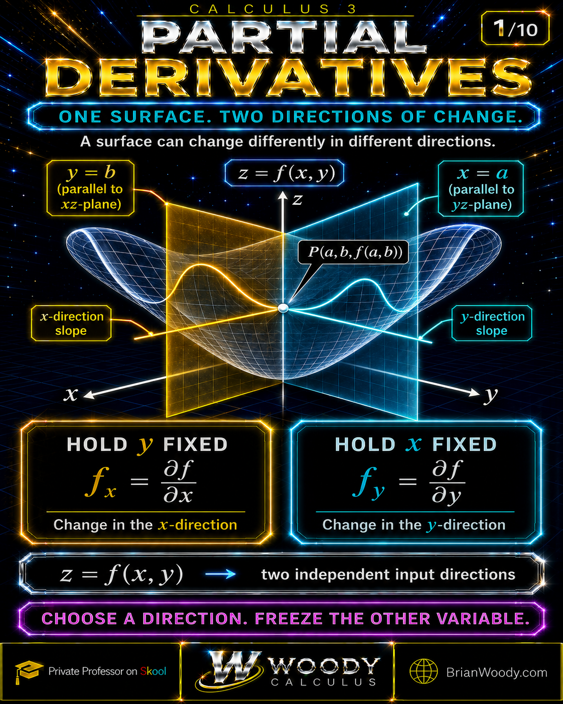
A partial derivative is the one-variable rate of change obtained by allowing one independent variable to move while every other independent variable remains fixed.
For a function of one variable, \(y=g(x)\), there is only one input direction. For a function of two variables, \(z=f(x,y)\), the input can move in the \(x\)-direction, the \(y\)-direction, or any combination of the two. The first partial derivatives isolate the two coordinate directions:
The x-partial
f_x(x,y)=\frac{\partial f}{\partial x}
\]
Vary \(x\), hold \(y\) fixed, and measure the slope of the resulting \(x\)-trace.
The y-partial
f_y(x,y)=\frac{\partial f}{\partial y}
\]
Vary \(y\), hold \(x\) fixed, and measure the slope of the resulting \(y\)-trace.
Why Are Partial Derivatives Slopes of Trace Curves?
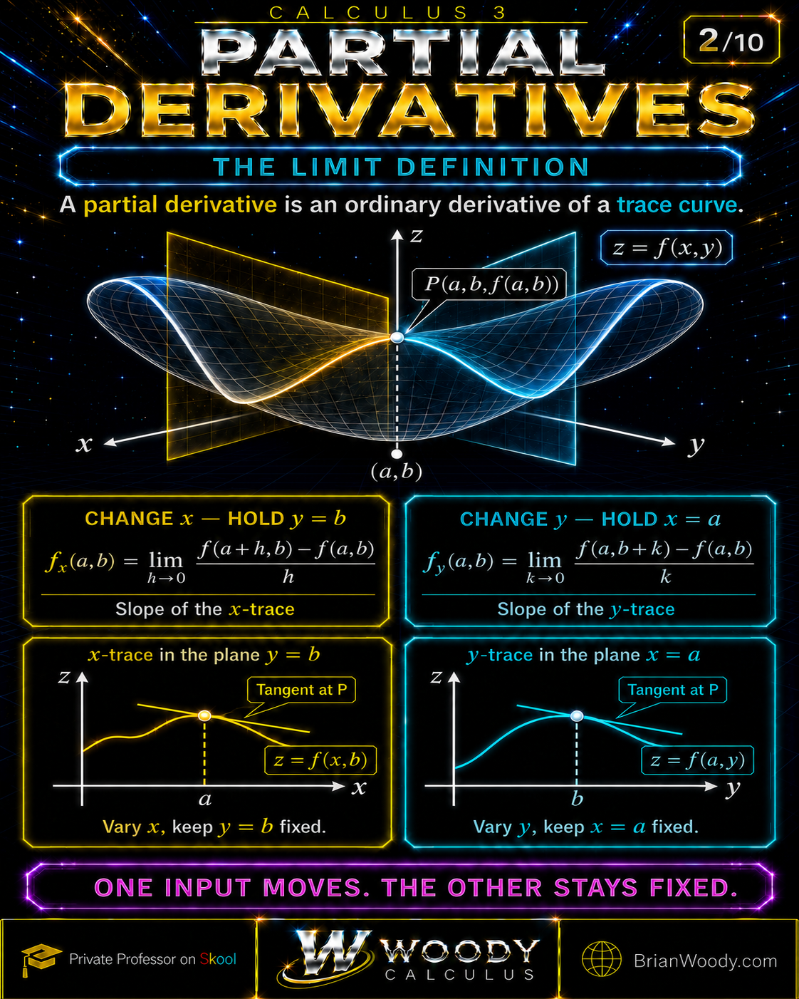
Fixing one input intersects the surface with a vertical plane, producing an ordinary one-variable curve whose derivative is the corresponding partial derivative.
At the surface point \(P(a,b,f(a,b))\), fixing \(y=b\) produces the trace \(z=f(x,b)\) in the plane \(y=b\). Its derivative at \(x=a\) is \(f_x(a,b)\). Fixing \(x=a\) produces the trace \(z=f(a,y)\) in the plane \(x=a\). Its derivative at \(y=b\) is \(f_y(a,b)\).
\[
f_x(a,b)=\lim_{h\to0}\frac{f(a+h,b)-f(a,b)}{h},
\qquad
f_y(a,b)=\lim_{k\to0}\frac{f(a,b+k)-f(a,b)}{k}.
\]
| Derivative | Variable that moves | Variable held fixed | Trace curve |
|---|---|---|---|
| \(f_x(a,b)\) | \(x\) | \(y=b\) | \(z=f(x,b)\) |
| \(f_y(a,b)\) | \(y\) | \(x=a\) | \(z=f(a,y)\) |
Partial Derivative Notation: How Do You Read ∂, \(f_x\), and \(\partial f/\partial x\)?
The symbol \(\partial\) identifies differentiation with respect to one variable in a multivariable function; several common notations express the same coordinate-direction derivative.
The symbol \(\partial\) is called the partial-derivative symbol and is often described as a “curly d.” It is not the Greek letter delta. The following three expressions usually mean the same first partial derivative:
| Notation | Read aloud | Meaning |
|---|---|---|
| \(\dfrac{\partial f}{\partial x}\) | “Partial \(f\) with respect to \(x\)” | Differentiate \(f\) with respect to \(x\), holding the other independent variables constant. |
| \(f_x\) | “\(f\) sub \(x\)” | A compact subscript notation for the same derivative. |
| \(D_xf\) | “\(D\) sub \(x\) of \(f\)” | Operator notation emphasizing differentiation in the \(x\)-coordinate direction. |
What changes when a function has three variables?
Nothing changes about the method. Choose one variable, freeze the other two, and differentiate. For
w(x,y,z)=x^2yz+e^{xz},
\]
the three first partial derivatives are
\boxed{w_x=2xyz+ze^{xz}},
\qquad
\boxed{w_y=x^2z},
\qquad
\boxed{w_z=x^2y+xe^{xz}}.
\]
For \(w_x\), both \(y\) and \(z\) are constant. For \(w_y\), both \(x\) and \(z\) are constant. For \(w_z\), both \(x\) and \(y\) are constant.
How Do You Find Partial Derivatives?
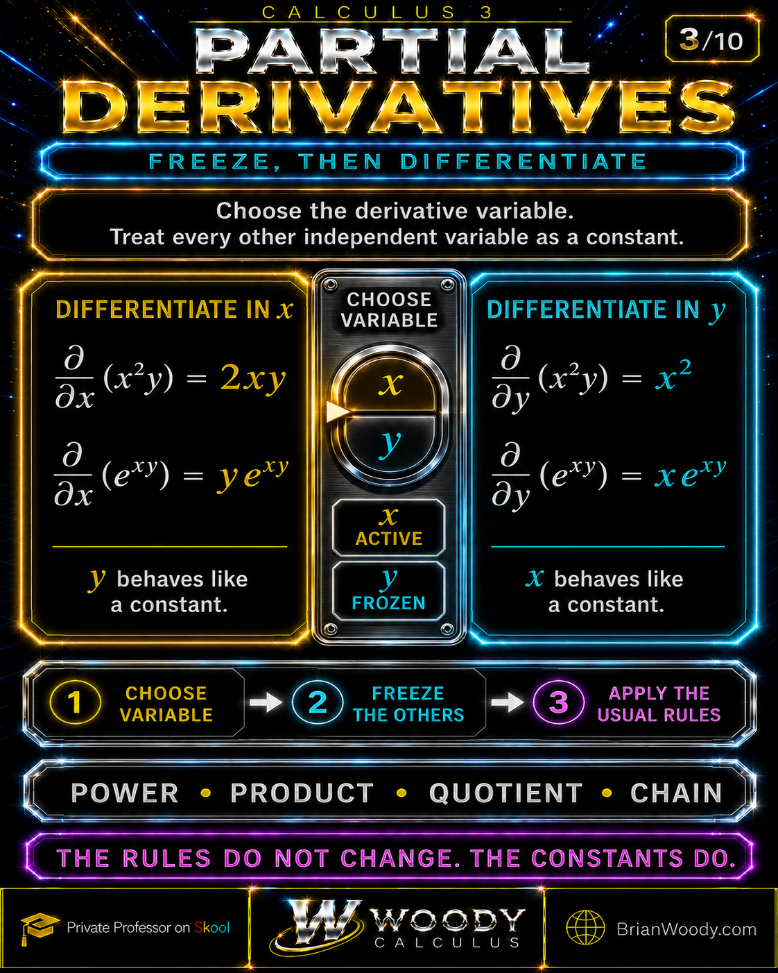
Use the same differentiation rules from single-variable calculus, but first decide which variable moves and which variables must be treated as constants.
-
Identify the independent variables
Write down every independent variable in the function and note which quantities depend on them.
-
Choose the differentiation variable
Use the notation in the problem to determine whether you need the x-partial, the y-partial, or another partial derivative.
-
Freeze every other independent variable
Treat all unselected independent variables as constants. Do not replace them with zero.
-
Differentiate using the usual rules
Apply the power, product, quotient, and chain rules exactly as you would in single-variable calculus.
-
Simplify the resulting function
Combine like terms, factor when useful, and preserve the derivative notation until the result is clear.
-
Evaluate at the requested point
Substitute the point after differentiating unless the problem gives a specific reason to do otherwise.
-
Interpret the result
State the direction, sign, magnitude, and units of the rate of change whenever the problem has context.
-
Verify mixed partials when justified
Compare mixed partials only after checking the continuity conditions required by Clairaut’s theorem.
Power-rule example
\frac{\partial}{\partial x}(x^2y)=2xy,
\qquad
\frac{\partial}{\partial y}(x^2y)=x^2.
\]
Chain-rule example
\frac{\partial}{\partial x}e^{xy}=ye^{xy},
\qquad
\frac{\partial}{\partial y}e^{xy}=xe^{xy}.
\]
Complete Worked Example: Find \(f_x\) and \(f_y\)
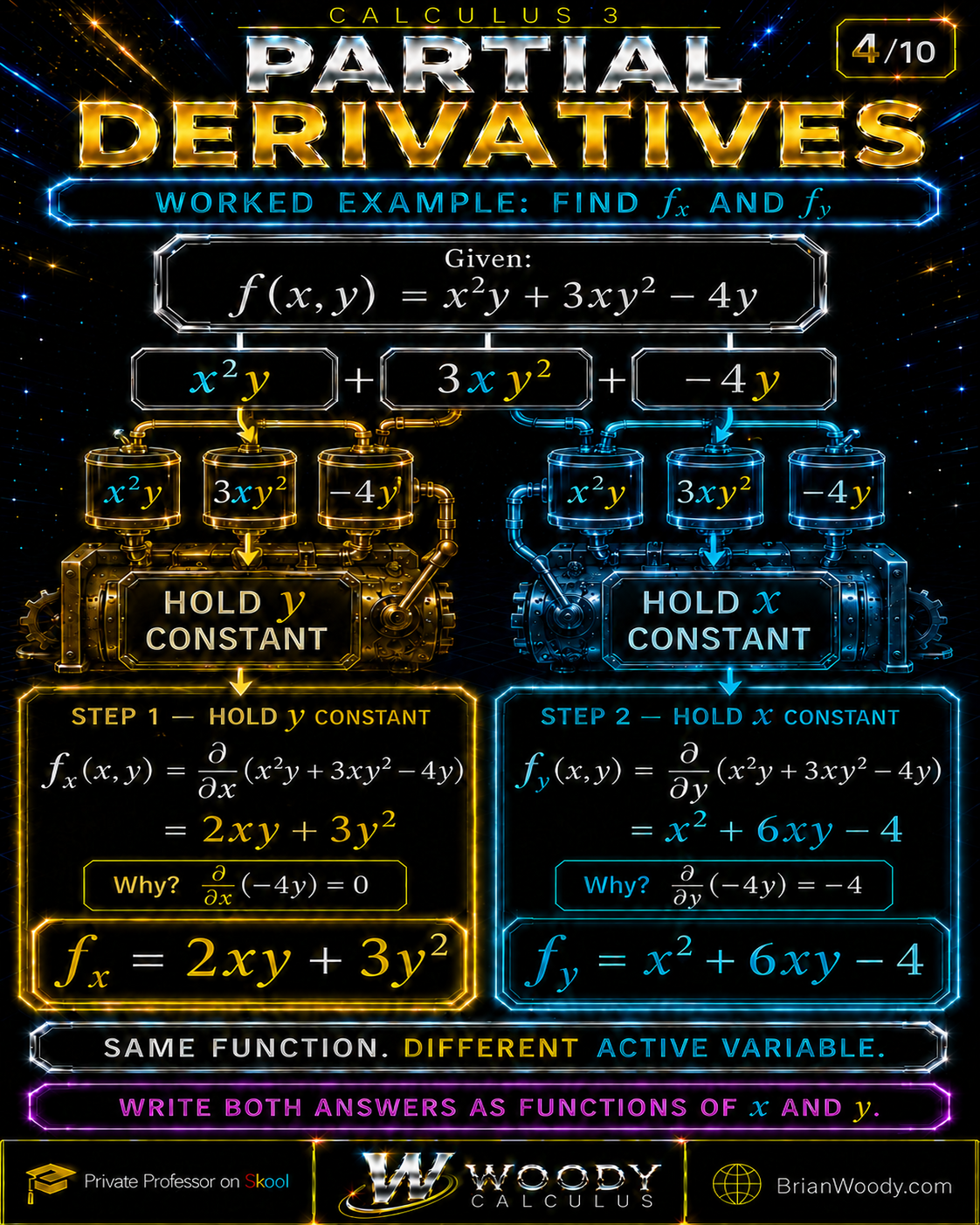
The safest way to compute first partial derivatives is to differentiate the function term by term while explicitly tracking which variable is frozen.
f(x,y)=x^2y+3xy^2-4y.
\]
Differentiate with respect to \(x\)
Hold \(y\) constant. The factor \(y\) behaves like a numerical coefficient, and the term \(-4y\) is constant with respect to \(x\).
\begin{aligned}
f_x(x,y)
&=\frac{\partial}{\partial x}\left(x^2y+3xy^2-4y\right)\\
&=2xy+3y^2+0\\
&=\boxed{2xy+3y^2}.
\end{aligned}
\]
Differentiate with respect to \(y\)
Hold \(x\) constant. The factor \(x^2\) is constant, \(3x\) is the coefficient of \(y^2\), and \(-4y\) contributes \(-4\).
\begin{aligned}
f_y(x,y)
&=\frac{\partial}{\partial y}\left(x^2y+3xy^2-4y\right)\\
&=x^2+6xy-4\\
&=\boxed{x^2+6xy-4}.
\end{aligned}
\]
How Do You Evaluate and Interpret a Partial Derivative?
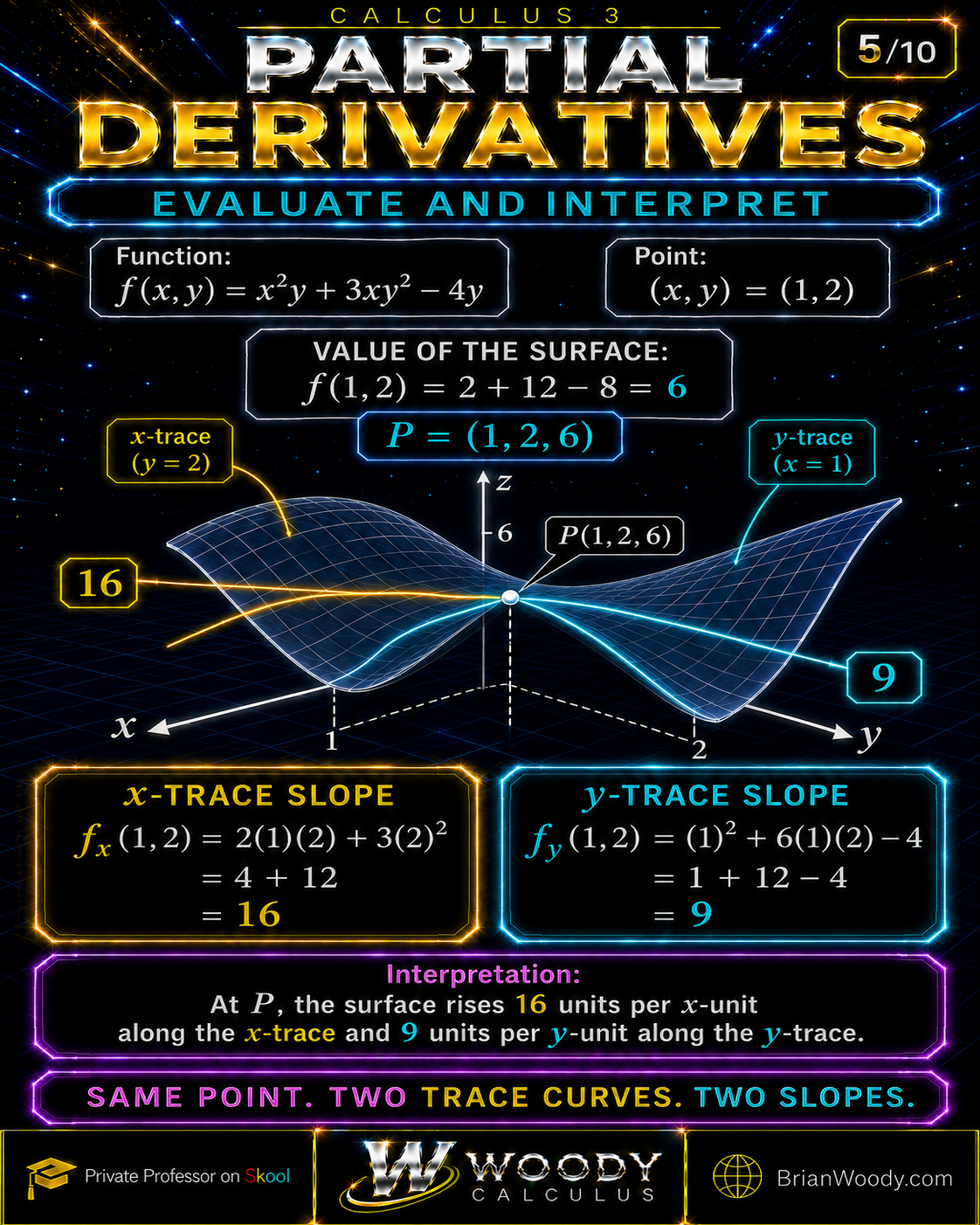
Differentiate first, then substitute the point; the resulting number is the slope of the appropriate trace curve at that surface point.
At \((1,2)\), the surface value is
f(1,2)=1^2(2)+3(1)(2^2)-4(2)=2+12-8=\boxed{6}.
\]
x-trace slope
f_x(1,2)=2(1)(2)+3(2^2)=4+12=\boxed{16}.
\]
y-trace slope
f_y(1,2)=1^2+6(1)(2)-4=1+12-4=\boxed{9}.
\]
At \(P=(1,2,6)\), the surface rises \(16\) vertical units per unit of \(x\) along the \(x\)-trace and \(9\) vertical units per unit of \(y\) along the \(y\)-trace.
Applied Partial Derivatives: Temperature Rates and Table Estimates
In an applied model, a partial derivative measures an output rate in one coordinate direction, and the same rate can be estimated from nearby table values when no formula is available.
Temperature-field example with units
Suppose the temperature on a flat plate is modeled by
T(x,y)=20+0.04x^2-0.03y^2,
\]
where \(T\) is measured in degrees Celsius and \(x\) and \(y\) are measured in meters. The coordinate-direction temperature rates are
T_x(x,y)=0.08x,
\qquad
T_y(x,y)=-0.06y.
\]
At \((5,10)\),
Rate in the positive \(x\)-direction
\boxed{T_x(5,10)=0.4\ ^\circ\mathrm C/\mathrm m}.
\]
Near this point, temperature increases by approximately \(0.4^\circ\mathrm C\) for each meter traveled in the positive \(x\)-direction while \(y\) stays fixed.
Rate in the positive \(y\)-direction
\boxed{T_y(5,10)=-0.6\ ^\circ\mathrm C/\mathrm m}.
\]
Near this point, temperature decreases by approximately \(0.6^\circ\mathrm C\) for each meter traveled in the positive \(y\)-direction while \(x\) stays fixed.
How do you estimate a partial derivative from a table?
If values are available on both sides of the point, use a central difference. With spacing \(h\),
\boxed{f_x(a,b)\approx\frac{f(a+h,b)-f(a-h,b)}{2h}},
\qquad
\boxed{f_y(a,b)\approx\frac{f(a,b+h)-f(a,b-h)}{2h}}.
\]
| \(y\backslash x\) | \(x=4\) | \(x=5\) | \(x=6\) |
|---|---|---|---|
| \(y=9\) | 18.21 | 18.57 | 19.01 |
| \(y=10\) | 17.64 | 18.00 | 18.44 |
| \(y=11\) | 17.01 | 17.37 | 17.81 |
Using \(h=1\), the table gives
T_x(5,10)\approx\frac{T(6,10)-T(4,10)}{2}
=\frac{18.44-17.64}{2}=\boxed{0.40\ ^\circ\mathrm C/\mathrm m},
\]
\[
T_y(5,10)\approx\frac{T(5,11)-T(5,9)}{2}
=\frac{17.37-18.57}{2}=\boxed{-0.60\ ^\circ\mathrm C/\mathrm m}.
\]
These central differences equal the exact derivatives here because the model is quadratic in each variable and the table values are exact.
What Are Second and Mixed Partial Derivatives?
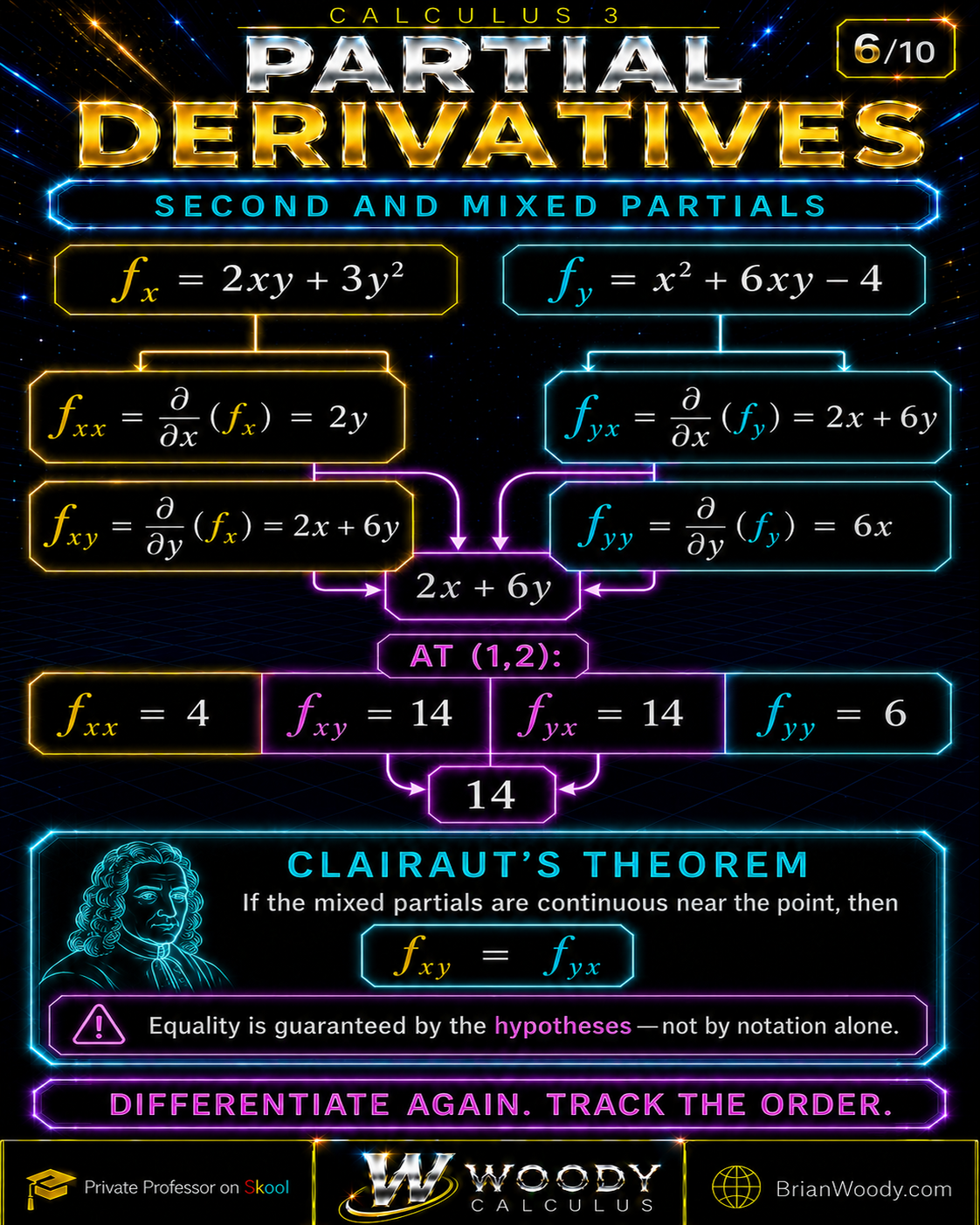
A second partial derivative differentiates a first partial again; the subscripts record the order of differentiation and must be read carefully.
Using the convention that \(f_{xy}\) means differentiate \(f_x\) with respect to \(y\), the running example gives
\begin{aligned}
f_{xx}&=\frac{\partial}{\partial x}(2xy+3y^2)=2y,\\
f_{xy}&=\frac{\partial}{\partial y}(2xy+3y^2)=2x+6y,\\
f_{yx}&=\frac{\partial}{\partial x}(x^2+6xy-4)=2x+6y,\\
f_{yy}&=\frac{\partial}{\partial y}(x^2+6xy-4)=6x.
\end{aligned}
\]
At \((1,2)\),
f_{xx}(1,2)=4,
\qquad
f_{xy}(1,2)=14,
\qquad
f_{yx}(1,2)=14,
\qquad
f_{yy}(1,2)=6.
\]
Clairaut’s theorem
If \(f_{xy}\) and \(f_{yx}\) are continuous on an open region containing \((a,b)\), then
\boxed{f_{xy}(a,b)=f_{yx}(a,b)}.
\]
This equality follows from the continuity hypotheses. It is not guaranteed by the notation alone.
Can the mixed partials be different?
Yes. Consider
F(x,y)=
\begin{cases}
\dfrac{xy(x^2-y^2)}{x^2+y^2},&(x,y)\ne(0,0),\\[6pt]
0,&(x,y)=(0,0).
\end{cases}
\]
Directly from the definitions, \(F_x(0,y)=-y\) and \(F_y(x,0)=x\). Therefore,
\boxed{F_{xy}(0,0)=-1}
\qquad\text{but}\qquad
\boxed{F_{yx}(0,0)=1}.
\]
The mixed partials disagree because the continuity conditions required by Clairaut’s theorem fail at the origin.
How Do Partial Derivatives Build a Tangent Plane?
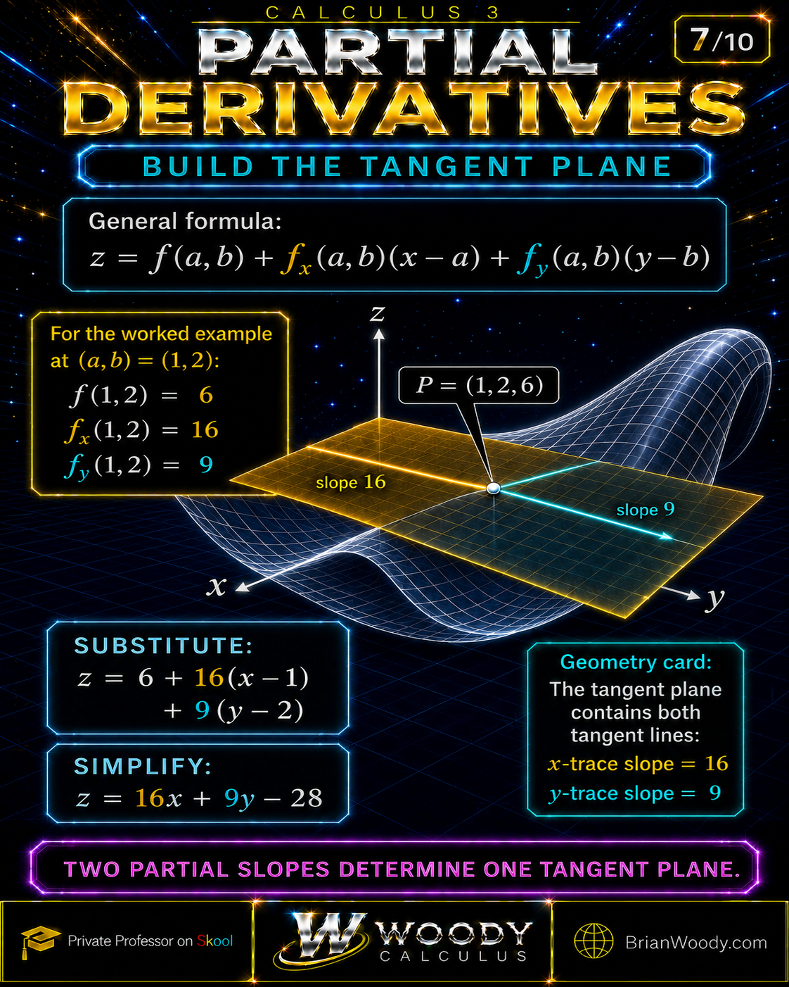
When \(f\) is differentiable at \((a,b)\), the two first partial derivatives determine the plane that best approximates the surface near \(P=(a,b,f(a,b))\).
\[
\boxed{z=f(a,b)+f_x(a,b)(x-a)+f_y(a,b)(y-b)}.
\]
For the running example at \((a,b)=(1,2)\),
\begin{aligned}
z&=6+16(x-1)+9(y-2)\\
&=\boxed{16x+9y-28}.
\end{aligned}
\]
Do existing partial derivatives guarantee a tangent plane?
No. The existence of \(f_x(a,b)\) and \(f_y(a,b)\) alone does not guarantee continuity or differentiability. Define
G(x,y)=
\begin{cases}
\dfrac{xy}{x^2+y^2},&(x,y)\ne(0,0),\\[6pt]
0,&(x,y)=(0,0).
\end{cases}
\]
Both partial derivatives at the origin exist and equal zero. However, along \(y=x\),
G(x,x)=\frac{x^2}{2x^2}=\frac12
\qquad (x\ne0),
\]
so \(G\) is not continuous at the origin and therefore is not differentiable there. A common sufficient condition is that the first partial derivatives exist and are continuous near the point.
How Does the Multivariable Chain Rule Use Partial Derivatives?
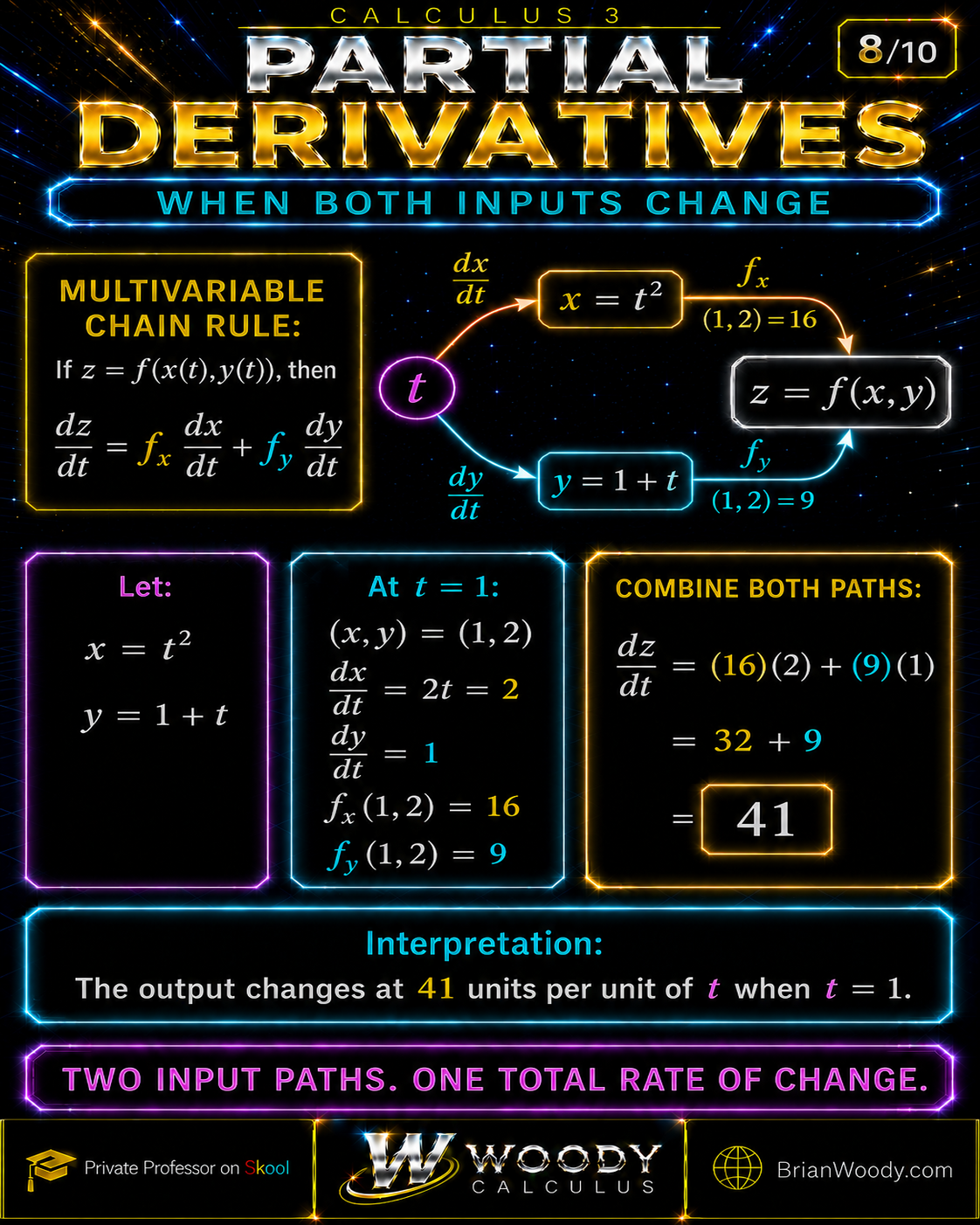
When every input changes with time, the total output rate is the sum of each partial derivative multiplied by the rate of its corresponding input.
\boxed{\frac{dz}{dt}=f_x(x(t),y(t))\frac{dx}{dt}+f_y(x(t),y(t))\frac{dy}{dt}}.
\]
Let \(z=f(x,y)\), \(x=t^2\), and \(y=1+t\). At \(t=1\),
(x,y)=(1,2),
\qquad
\frac{dx}{dt}=2t=2,
\qquad
\frac{dy}{dt}=1.
\]
Since \(f_x(1,2)=16\) and \(f_y(1,2)=9\),
\frac{dz}{dt}=16(2)+9(1)=32+9=\boxed{41}.
\]
The derivative is one linear map
At \((1,2)\), the derivative of \(f\) can be represented by the row matrix
Df(1,2)=\begin{bmatrix}16&9\end{bmatrix}.
\]
Applying this linear map to the input velocity gives the chain-rule result:
Df(1,2)
\begin{bmatrix}2\\1\end{bmatrix}
=\begin{bmatrix}16&9\end{bmatrix}
\begin{bmatrix}2\\1\end{bmatrix}
=41.
\]
The same vector of partial derivatives is the gradient:
\nabla f(1,2)=\langle16,9\rangle.
\]
Continue this connection in the Woody Calculus lesson on gradient and directional derivatives.
How Partial Derivatives Power Implicit Differentiation and PDEs
Partial derivatives extend the chain rule to implicitly defined curves and provide the basic language for differential equations involving more than one independent variable.
Implicit differentiation with partial derivatives
Suppose a curve is defined implicitly by \(F(x,y)=0\), where \(y=y(x)\). Differentiating the constant relation with respect to \(x\) gives
0=\frac{d}{dx}F(x,y(x))=F_x+F_y\frac{dy}{dx}.
\]
Therefore, wherever \(F_y\ne0\),
\boxed{\frac{dy}{dx}=-\frac{F_x}{F_y}}.
\]
For the circle \(F(x,y)=x^2+y^2-25=0\),
F_x=2x,
\qquad
F_y=2y,
\qquad
\frac{dy}{dx}=-\frac{x}{y}.
\]
\[
\left.\frac{dy}{dx}\right|_{(3,4)}=\boxed{-\frac34}.
\]
The condition \(F_y(3,4)=8\ne0\) confirms that the circle can be represented locally as a differentiable function \(y=y(x)\) near \((3,4)\).
Verify a solution of a partial differential equation
A partial differential equation, or PDE, relates a multivariable function to its partial derivatives. Consider the one-dimensional heat equation
u_t=u_{xx}.
\]
To test \(u(x,t)=e^{-4t}\sin(2x)\), differentiate in the required directions:
u_t=-4e^{-4t}\sin(2x),
\]
\[
u_x=2e^{-4t}\cos(2x),
\qquad
u_{xx}=-4e^{-4t}\sin(2x).
\]
Because \(u_t=u_{xx}\) for every \((x,t)\), the proposed function satisfies the heat equation. This is the same differentiation process used earlier; the notation simply tracks which independent variable is active.
How Do Partial Derivatives Estimate Small Changes?
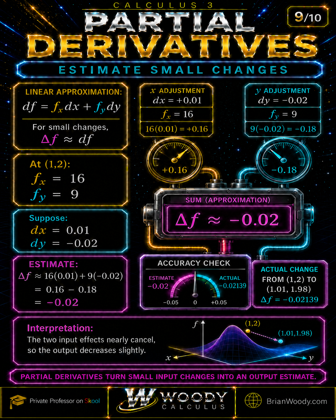
Near a differentiable point, the total differential combines the independent input changes into the best first-order estimate of the output change.
\boxed{df=f_x(a,b)\,dx+f_y(a,b)\,dy}
\qquad\text{and}\qquad
\boxed{\Delta f\approx df}.
\]
Move from \((1,2)\) to \((1.01,1.98)\). Then \(dx=0.01\) and \(dy=-0.02\), so
\begin{aligned}
df&=16(0.01)+9(-0.02)\\
&=0.16-0.18\\
&=\boxed{-0.02}.
\end{aligned}
\]
The actual change is
\Delta f=f(1.01,1.98)-f(1,2)=5.97861-6=\boxed{-0.02139}.
\]
Why is the estimate off by about \(0.00139\)?
The first-order differential ignores curvature. At \((1,2)\), the Hessian matrix is
H_f(1,2)=
\begin{bmatrix}
f_{xx}&f_{xy}\\
f_{yx}&f_{yy}
\end{bmatrix}_{(1,2)}
=
\begin{bmatrix}
4&14\\
14&6
\end{bmatrix}.
\]
For \(\Delta\mathbf x=\langle0.01,-0.02\rangle\), the quadratic Taylor correction is
\frac12\Delta\mathbf x^{T}H_f(1,2)\Delta\mathbf x=-0.0014.
\]
Thus the second-order estimate is \(-0.02-0.0014=-0.0214\), already within \(0.00001\) of the exact change. Because the function is cubic, its third-order term contributes the remaining \(0.00001\), producing the exact value \(-0.02139\).
Partial Derivatives Decision Map
The reliable exam process is to identify the independent variables, choose the differentiation variable, freeze the others, differentiate, simplify, evaluate, interpret, and verify any theorem hypotheses before drawing a conclusion.
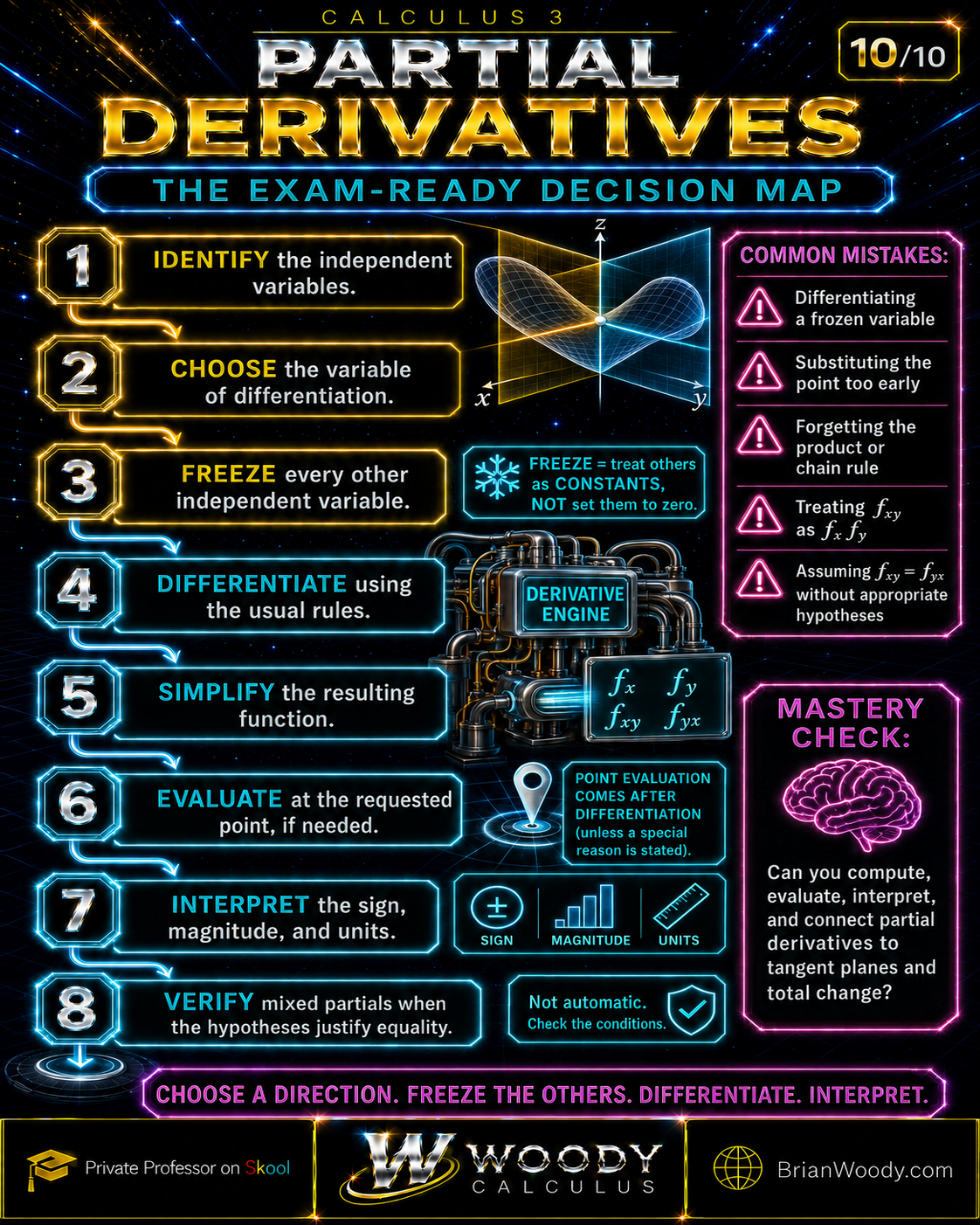
List the independent variables.
Select the differentiation variable.
Treat the other inputs as constants.
Use the ordinary derivative rules.
Organize the resulting function.
Substitute the requested point.
State sign, magnitude, direction, and units.
Check computations and theorem hypotheses.
Common Partial Derivative Mistakes
Most errors come from mishandling the frozen variables, substituting too early, or applying a theorem without checking its hypotheses.
Setting a frozen variable equal to zero
Fix: treat it as an arbitrary constant. In \(\partial(x^2y)/\partial x\), the factor \(y\) remains, giving \(2xy\).
Differentiating a frozen variable
Fix: when finding \(f_x\), any expression involving only \(y\) has derivative zero with respect to \(x\).
Substituting the point too early
Fix: find the partial derivative function first, then evaluate it at the requested point.
Forgetting the product or chain rule
Fix: the derivative rules do not change. For example, \(\partial e^{xy}/\partial x=ye^{xy}\).
Reading mixed-partial subscripts backward
Fix: state your convention. In this lesson, \(f_{xy}\) means differentiate \(f_x\) with respect to \(y\).
Assuming mixed partials always agree
Fix: use Clairaut’s theorem only when the required continuity hypotheses hold near the point.
Assuming existing partials imply differentiability
Fix: partial derivatives can exist even when the function is not continuous. Check a differentiability theorem or the definition.
Reporting a number without meaning or units
Fix: identify the trace direction and write output units per unit of the selected input.
Partial Derivatives Practice Problems with Solutions
Use these problems to train computation, evaluation, interpretation, tangent planes, the chain rule, linear approximation, three-variable derivatives, implicit differentiation, table estimates, PDE verification, and the logical limits of the theory.
1. Find both first partial derivatives of \(g(x,y)=x^3y^2-5xe^y\).
For \(g_x\), hold \(y\) constant. For \(g_y\), hold \(x\) constant:
\boxed{g_x=3x^2y^2-5e^y},
\qquad
\boxed{g_y=2x^3y-5xe^y}.
\]
2. Find and evaluate the partial derivatives of \(h(x,y)=\ln(x^2+y^2)\) at \((1,2)\).
Apply the chain rule, noting that the function is defined away from \((0,0)\):
h_x=\frac{2x}{x^2+y^2},
\qquad
h_y=\frac{2y}{x^2+y^2}.
\]
\[
\boxed{h_x(1,2)=\frac25},
\qquad
\boxed{h_y(1,2)=\frac45}.
\]
3. Find \(p_x\) and \(p_y\) for \(p(x,y)=x^2\sin y+ye^x\).
\boxed{p_x=2x\sin y+ye^x},
\qquad
\boxed{p_y=x^2\cos y+e^x}.
\]
The term \(ye^x\) requires different reasoning in the two directions: \(y\) is constant for \(p_x\), while \(e^x\) is constant for \(p_y\).
4. Verify that the mixed partials agree for \(q(x,y)=x^2y+e^{xy}\).
q_x=2xy+ye^{xy},
\qquad
q_y=x^2+xe^{xy}.
\]
\[
\boxed{q_{xy}=2x+(1+xy)e^{xy}=q_{yx}}.
\]
Because this function has continuous partial derivatives of every order on \(\mathbb R^2\), Clairaut’s theorem applies everywhere.
5. Find the tangent plane to \(z=x^2+y^2\) at \((1,2,5)\).
Here \(f_x=2x\) and \(f_y=2y\), so \(f_x(1,2)=2\) and \(f_y(1,2)=4\):
z=5+2(x-1)+4(y-2)=\boxed{2x+4y-5}.
\]
6. For the running example, let \(x=t^2\) and \(y=1+t\). Find \(dz/dt\) at \(t=1\).
At \(t=1\), \((x,y)=(1,2)\), \(dx/dt=2\), and \(dy/dt=1\). Therefore,
\frac{dz}{dt}=f_x\frac{dx}{dt}+f_y\frac{dy}{dt}=16(2)+9(1)=\boxed{41}.
\]
7. Use linear approximation to estimate \(\sqrt{3.02^2+3.99^2}\).
Let \(r(x,y)=\sqrt{x^2+y^2}\) and linearize at \((3,4)\), where \(r=5\), \(r_x=3/5\), and \(r_y=4/5\). With \(dx=0.02\) and \(dy=-0.01\),
dr=\frac35(0.02)+\frac45(-0.01)=0.012-0.008=0.004.
\]
\[
\boxed{\sqrt{3.02^2+3.99^2}\approx5.004}.
\]
8. Can a function have both partial derivatives at a point and still fail to be differentiable there?
Yes. For \(G(x,y)=xy/(x^2+y^2)\) away from the origin and \(G(0,0)=0\), both first partial derivatives at the origin equal zero. However, \(G(x,x)=1/2\) for every nonzero \(x\), so \(G\) is not continuous at the origin and cannot be differentiable there.
9. Find all three first partial derivatives of \(v(x,y,z)=xyz^2+\cos(yz)\).
Differentiate with respect to one variable at a time while holding the other two constant:
\boxed{v_x=yz^2},
\qquad
\boxed{v_y=xz^2-z\sin(yz)},
\qquad
\boxed{v_z=2xyz-y\sin(yz)}.
\]
10. Estimate \(f_x(2,3)\) from \(f(1.9,3)=7.41\) and \(f(2.1,3)=7.81\).
The values lie symmetrically around \(x=2\), with \(h=0.1\). Use the central difference:
f_x(2,3)\approx\frac{f(2.1,3)-f(1.9,3)}{2(0.1)}
=\frac{7.81-7.41}{0.2}=\boxed{2}.
\]
11. Use partial derivatives to find \(dy/dx\) for \(x^2+xy+y^2=7\) at \((1,2)\).
Let \(F(x,y)=x^2+xy+y^2-7\). Then \(F_x=2x+y\) and \(F_y=x+2y\). Because \(F_y(1,2)=5\ne0\),
\frac{dy}{dx}=-\frac{F_x}{F_y}
=-\frac{2x+y}{x+2y},
\qquad
\left.\frac{dy}{dx}\right|_{(1,2)}
=-\frac{4}{5}=\boxed{-\frac45}.
\]
12. Verify that \(u(x,t)=e^{-9t}\sin(3x)\) satisfies \(u_t=u_{xx}\).
u_t=-9e^{-9t}\sin(3x),
\qquad
u_x=3e^{-9t}\cos(3x),
\]
\[
u_{xx}=-9e^{-9t}\sin(3x)=u_t.
\]
Therefore, the proposed function satisfies the heat equation for every \((x,t)\).
Partial Derivatives Glossary
These definitions collect the essential vocabulary connecting partial derivatives to geometry, approximation, and later topics in multivariable calculus.
- Partial derivative
- The rate of change of a multivariable function with respect to one independent variable while the others are held constant.
- Partial-derivative symbol
- The symbol \(\partial\), commonly read as “partial” or described as a curly d, used in notation such as \(\partial f/\partial x\).
- x-partial
- The derivative \(f_x\), obtained by differentiating with respect to \(x\) while treating the other independent variables as constants.
- y-partial
- The derivative \(f_y\), obtained by differentiating with respect to \(y\) while treating the other independent variables as constants.
- Trace curve
- A curve formed by intersecting a surface with a plane such as \(x=a\) or \(y=b\).
- Mixed partial derivative
- A higher-order derivative taken with respect to more than one independent variable, such as \(f_{xy}\) or \(f_{yx}\).
- Tangent plane
- The plane that gives the best first-order approximation to a differentiable surface near a point.
- Linear approximation
- The local approximation of a differentiable function by its tangent plane or derivative linear map.
- Total differential
- The first-order change \(df=f_xdx+f_ydy\) generated by small changes in the independent variables.
- Multivariable chain rule
- A rule that combines partial derivatives with the rates at which the independent variables change.
- Gradient
- The vector of first partial derivatives, \(\nabla f=\langle f_x,f_y\rangle\), which points in the direction of steepest increase.
- Hessian matrix
- The square matrix of second partial derivatives used to describe curvature and second-order approximation.
- Differentiability
- The property that a function has a valid local linear approximation with an error that is small relative to the input displacement.
- Central difference
- A symmetric numerical estimate of a derivative that uses function values on both sides of the point.
- Implicit differentiation
- A chain-rule method for differentiating a relation such as \(F(x,y)=0\) without first solving explicitly for one variable.
- Partial differential equation
- An equation involving an unknown function of several independent variables and one or more of its partial derivatives.
Frequently Asked Questions About Partial Derivatives
These concise answers address the questions students most often ask about notation, computation, geometry, differentiability, and applications.
What is a partial derivative?
A partial derivative measures how a multivariable function changes with respect to one independent variable while every other independent variable is held constant.
How do you calculate a partial derivative?
Choose the differentiation variable, treat every other independent variable as a constant, and apply the usual power, product, quotient, and chain rules.
What is the difference between an ordinary derivative and a partial derivative?
An ordinary derivative differentiates a function with one independent variable. A partial derivative differentiates a multivariable function in one selected input direction.
What does holding a variable constant mean?
Holding a variable constant means treating it as a fixed coefficient during differentiation. It does not mean replacing that variable with zero.
Do existing partial derivatives guarantee continuity or differentiability?
No. A function can have both first partial derivatives at a point and still fail to be continuous or differentiable there.
When are the mixed partial derivatives equal?
Clairaut’s theorem guarantees equality when the relevant mixed partial derivatives are continuous on an open region containing the point.
What is the tangent-plane formula?
At a differentiable point, the tangent plane equals the function value plus the x-partial times the change in x plus the y-partial times the change in y.
What is the multivariable chain rule?
When x and y depend on time, the total rate is the x-partial times dx over dt plus the y-partial times dy over dt.
How are partial derivatives related to the gradient?
The gradient is the vector formed from the first partial derivatives. For a two-variable function, its components are the x-partial and y-partial.
What units does a partial derivative have?
A partial derivative has units of the function’s output divided by the units of the selected independent variable.
What is the ∂ symbol called?
The symbol ∂ is called the partial-derivative symbol and is often described as a curly d. It indicates differentiation with respect to one variable of a multivariable function.
Can you estimate partial derivatives from a table?
Yes. Hold the other input fixed and use nearby values in the selected direction; when values are available on both sides, a central difference usually gives the best elementary estimate.
How are partial derivatives used in implicit differentiation and PDEs?
For an implicit relation, partial derivatives combine through the chain rule to determine the slope of the curve. In a partial differential equation, they describe how an unknown multivariable function changes in different independent-variable directions.
References and Further Reading
These openly available references support the definitions, tangent-plane formulas, chain rule, numerical differentiation, gradient connections, and introductory PDE verification used in this lesson.
- OpenStax Calculus Volume 3, Section 4.3: Partial Derivatives
- OpenStax Calculus Volume 3, Section 4.4: Tangent Planes and Linear Approximations
- OpenStax Calculus Volume 3, Section 4.5: The Chain Rule
- OpenStax Calculus Volume 3, Section 4.6: Directional Derivatives and the Gradient
- NIST Digital Library of Mathematical Functions, Section 3.4: Numerical Differentiation
- MIT OpenCourseWare 18.303: Linear Partial Differential Equations