LINEAR ALGEBRA • COMPLETE THEOREM ATLAS • 50 EQUIVALENT CONDITIONS
The Invertible Matrix Theorem is the master connection map of a first linear algebra course. It says that row reduction, pivots, null spaces, bases, systems of equations, linear transformations, determinants, eigenvalues, singular values, and geometry are not isolated chapters. For a square matrix, they are different languages describing the same mathematical reality.
This lesson develops that reality from the ground up. You can use it as a first encounter, a proof guide, an exam reference, or a map showing how the fundamentals of linear algebra fit together.
Reading time: approximately 55–70 minutes for the complete lesson; 8–12 minutes for the direct answer, quick atlas, and test guide.
What Is the Invertible Matrix Theorem?
Let \(A\in\mathbb R^{n\times n}\) be a square matrix, and let \(T:\mathbb R^n\to\mathbb R^n\) be the linear transformation \(T(x)=Ax\). The Invertible Matrix Theorem says that many conditions are equivalent: \(A\) has an inverse; \(\operatorname{rref}(A)=I_n\); \(A\) has a pivot in every row and column; \(Ax=0\) has only the trivial solution; the columns form a basis of \(\mathbb R^n\); \(Ax=b\) has exactly one solution for every \(b\); \(T\) is one-to-one and onto; \(\det(A)\ne0\); zero is not an eigenvalue; every singular value is positive; and \(A^TA\) is positive definite.
“Equivalent” means all true or all false. Proving any one condition proves every condition in the theorem. Showing that any one fails proves that \(A\) is singular and every invertibility condition fails.
Quick Summary
- The theorem applies to a square matrix \(A\in\mathbb R^{n\times n}\).
- An invertible matrix preserves all \(n\) independent directions; a singular matrix loses at least one direction.
- Full pivots, trivial null space, independent columns, spanning columns, full rank, unique solvability, bijectivity, nonzero determinant, no zero eigenvalue, and positive smallest singular value are equivalent.
- The “one-to-one” and “onto” tests become equivalent because the domain and codomain have the same finite dimension.
- The determinant gives an exact yes/no test; the smallest singular value adds a numerical safety margin.
- An invertible matrix can still be ill-conditioned. Exact invertibility and numerical reliability are different questions.
- MathWorld presents 23 numbered classical conditions, but there is no universal maximum. This lesson organizes 50 useful, independently searchable formulations into one teaching atlas.
Memory sentence: Full pivots mean no direction is lost. Therefore the kernel is trivial, the image is the whole space, every system has one solution, the determinant and all singular values are nonzero, and the transformation can be reversed.
How to Test a Matrix for Invertibility
- Confirm that the matrix is square. The full Invertible Matrix Theorem requires A to be n by n. For rectangular matrices, separate full-column-rank and full-row-rank tests.
- Use the cheapest decisive information. Choose row reduction, a determinant, a known null space, eigenvalues, singular values, or transformation properties according to what the problem already gives.
- Test one equivalent condition. For example, establish n pivots, det(A) not zero, Nul(A) = {0}, zero absent from the spectrum, or σ_min(A) > 0.
- Invoke the theorem explicitly. State that because A is square and the tested condition holds, A is invertible and every equivalent IMT condition follows.
- Translate to the language the problem asks for. Convert invertibility into the requested conclusion about bases, systems, rank, one-to-one or onto maps, determinants, eigenvalues, or geometry.
- If one condition fails, switch to the singular world. A missing pivot, nonzero null vector, zero determinant, zero eigenvalue, or zero singular value makes every invertibility condition false.
- Check numerical conditioning separately. After exact invertibility is established, use singular values or a condition number to decide whether computation is stable.
Table of Contents
- The theorem, the count, and the two worlds
- The square-matrix hypothesis
- The complete 50-condition atlas
- Inverse, row reduction, pivots, and elementary matrices
- Null space, independence, spanning, bases, rank, and nullity
- Systems, existence, uniqueness, one-to-one, and onto
- Determinants, geometry, eigenvalues, and polynomials
- Rows, transpose, and the four fundamental subspaces
- SVD, Gram matrices, lower bounds, and conditioning
- Complete invertible and singular examples
- The proof network: why everything implies everything
- Fastest tests, applications, mistakes, and mastery
- Linear algebra reference dictionary
- Implication recipes and solved practice
- Frequently asked questions
Part I — The Theorem, the Count, and the Two Worlds

Why this may be the first theorem to learn
A typical linear algebra course introduces ideas one at a time: elimination, vector spaces, transformations, determinants, eigenvalues, orthogonality, and perhaps singular values. That sequence is necessary, but it can make the subject feel fragmented. The Invertible Matrix Theorem supplies the missing architecture.
Every major condition answers one of two deeper questions:
- Does \(A\) destroy information? This is the kernel, independence, injectivity, smallest-singular-value side.
- Can \(A\) reach every target? This is the column space, spanning, consistency, surjectivity side.
For a square map \(\mathbb R^n\to\mathbb R^n\), these questions have the same answer. If no direction is lost, all \(n\) output directions remain available. If every output is reachable, there is no room for two inputs to produce the same output. That equality of dimensions is the engine behind the theorem.
Are there 9, 23, 24, or 50 conditions?
All of those counts can be defensible because authors group statements differently. Some textbooks give a compact core of 8–12 conditions. MathWorld’s Invertible Matrix Theorem presents 23 numbered conditions equivalent to the ambient statement that \(A\) is invertible. Counting that ambient statement separately produces 24 propositions.
This lesson uses a declared teaching rule: it counts 50 pedagogically useful and independently searchable formulations. Some are close vocabulary restatements—such as \(\operatorname{Nul}(A)=\{0\}\) and \(\operatorname{nullity}(A)=0\)—because students encounter and search for both. There is no universal largest number: infinitely many equivalent statements can be manufactured.
The all-true-or-all-false principle
![Comparison of the invertible matrix A equals [[2,1],[1,1]] with determinant one and the singular matrix B equals [[2,4],[1,2]] with determinant zero, showing a unit square preserved as a parallelogram or collapsed to a line.](https://k3p6r8v3.delivery.rocketcdn.me/wp-content/uploads/2026/08/Invertible_Matrix_Theorem_Slide_02.png "Invertible or Singular — The Two Worlds of Square Matrices")
For
A=\begin{bmatrix}2&1\\1&1\end{bmatrix},
\qquad \det(A)=1,
\]
every condition in the atlas is true. The matrix has two pivots, trivial null space, rank two, a two-sided inverse, nonzero eigenvalues, positive singular values, and a transformation that is one-to-one and onto.
For
B=\begin{bmatrix}2&4\\1&2\end{bmatrix},
\qquad \det(B)=0,
\]
every condition is false. Its second column is twice its first; \(B[-2,1]^T=0\); rank is one; zero is an eigenvalue and singular value; and the map collapses the plane onto a line.
This binary split is the practical power of the theorem. You do not need to verify fifty statements. Find the cheapest decisive test available, then invoke equivalence.
Part II — The Square-Matrix Hypothesis
The standard theorem assumes
A\in\mathbb R^{n\times n},\qquad T:\mathbb R^n\longrightarrow\mathbb R^n.
\]
The word square is not a technicality. It makes row conditions and column conditions meet in the middle.
What changes for rectangular matrices?
Consider a \(3\times2\) matrix \(C\). It can have a pivot in every column and define a one-to-one map \(\mathbb R^2\to\mathbb R^3\), yet it cannot be onto \(\mathbb R^3\) because two input directions cannot span three output dimensions.
Now consider a \(2\times3\) matrix \(D\). It can have a pivot in every row and define an onto map \(\mathbb R^3\to\mathbb R^2\), yet it cannot be one-to-one because rank–nullity forces a nontrivial kernel.
| Matrix shape | Maximum useful pivot statement | Possible map behavior | Inverse behavior |
|---|---|---|---|
| \(n\times n\) | Pivot in every row and column | One-to-one iff onto | A one-sided inverse is automatically the two-sided inverse |
| \(m\times n\), (m>n) | Pivot in every column | Can be one-to-one, cannot be onto \(\mathbb R^m\) | May have a left inverse, not a right inverse |
| \(m\times n\), (m<n) | Pivot in every row | Can be onto, cannot be one-to-one | May have a right inverse, not a left inverse |
The Moore–Penrose pseudoinverse is useful for rectangular and rank-deficient matrices, but it is not an ordinary two-sided inverse and does not make the square IMT statements true.
What changes over the complex numbers?
The algebraic core works over any field with suitable language. Over \(\mathbb C\), replace the transpose by the conjugate transpose in inner-product statements:
A^TA\quad\text{becomes}\quad A^*A.
\]
Then \(x^*A^*Ax=\|Ax\|_2^2\), and the positive-definite Gram-matrix formulation remains correct.
Part III — The Complete 50-Condition Atlas
Every statement in the following atlas is equivalent for \(A\in\mathbb R^{n\times n}\). The “why it matches” column is intentionally short: use it for fast review, then visit the detailed family sections for proofs and examples.
| # | Family | Equivalent condition | Why it matches invertibility |
|---|---|---|---|
| 1 | A Inverse, elimination, and pivots | A is invertible (nonsingular). | The defining condition: a two-sided inverse exists. |
| 2 | A Inverse, elimination, and pivots | A is row-equivalent to In. | Reversible row operations carry A to the identity. |
| 3 | A Inverse, elimination, and pivots | rref(A) = In. | The unique reduced row-echelon form has every standard pivot. |
| 4 | A Inverse, elimination, and pivots | A has exactly n pivot positions. | Full rank leaves no missing direction. |
| 5 | A Inverse, elimination, and pivots | There is a pivot in every row. | Every output coordinate direction is reached. |
| 6 | A Inverse, elimination, and pivots | There is a pivot in every column. | No variable is free and no input direction is lost. |
| 7 | B Kernel, columns, and rank | Ax = 0 has only the solution x = 0. | No nonzero input is collapsed to zero. |
| 8 | B Kernel, columns, and rank | Nul(A) = {0}. | The kernel is trivial. |
| 9 | B Kernel, columns, and rank | nullity(A) = 0. | The kernel has dimension zero. |
| 10 | B Kernel, columns, and rank | The columns of A are linearly independent. | Only the trivial column combination equals zero. |
| 11 | B Kernel, columns, and rank | The columns of A span ℝn. | Every target is a column combination. |
| 12 | B Kernel, columns, and rank | The columns of A form a basis for ℝn. | They are both independent and spanning. |
| 13 | B Kernel, columns, and rank | Col(A) = ℝn. | The image is the entire codomain. |
| 14 | B Kernel, columns, and rank | dim Col(A) = n. | The image has full dimension. |
| 15 | B Kernel, columns, and rank | rank(A) = n. | The matrix has full rank. |
| 16 | C Rows and transpose | The rows of A are linearly independent. | They are the independent columns of A transpose. |
| 17 | C Rows and transpose | The rows of A span ℝn. | Full row rank reaches the whole row-coordinate space. |
| 18 | C Rows and transpose | The rows of A form a basis for ℝn. | n independent or spanning rows form a basis. |
| 19 | C Rows and transpose | Row(A) = ℝn. | The row space has full dimension. |
| 20 | C Rows and transpose | AT is invertible. | Rank is unchanged by transpose. |
| 21 | C Rows and transpose | Nul(AT) = {0}. | There is no nonzero left-null-space obstruction. |
| 22 | C Rows and transpose | nullity(AT) = 0. | The left null space has dimension zero. |
| 23 | D Systems and transformations | Ax = b is consistent for every b in ℝn. | Every target lies in the column space. |
| 24 | D Systems and transformations | Ax = b has exactly one solution for every b in ℝn. | Existence and uniqueness both hold globally. |
| 25 | D Systems and transformations | T(x) = Ax is one-to-one (injective). | Equal outputs force equal inputs. |
| 26 | D Systems and transformations | T(x) = Ax is onto ℝn (surjective). | Every output has a preimage. |
| 27 | D Systems and transformations | T(x) = Ax is bijective. | The map is both one-to-one and onto. |
| 28 | D Systems and transformations | T has an inverse linear transformation. | The input can be recovered linearly from every output. |
| 29 | D Systems and transformations | There is a matrix B with BA = In. | A left inverse forces injectivity and, for square A, invertibility. |
| 30 | D Systems and transformations | There is a matrix C with AC = In. | A right inverse forces surjectivity and, for square A, invertibility. |
| 31 | E Elementary matrices and subspaces | A is a product of elementary matrices. | A is assembled from reversible row operations. |
| 32 | E Elementary matrices and subspaces | Col(A)⊥ = {0}. | Its orthogonal complement is Nul(AT), which is trivial. |
| 33 | E Elementary matrices and subspaces | Nul(A)⊥ = ℝn. | The orthogonal complement of a zero kernel is the whole space. |
| 34 | F Determinant, spectrum, and polynomials | det(A) ≠ 0. | The determinant detects full rank and nonzero volume. |
| 35 | F Determinant, spectrum, and polynomials | Zero is not an eigenvalue of A. | No nonzero eigenvector can be sent to zero. |
| 36 | F Determinant, spectrum, and polynomials | pA(0) ≠ 0 for pA(t) = det(tI – A). | pA(0) = (-1)n det(A). |
| 37 | F Determinant, spectrum, and polynomials | The minimal polynomial mA has mA(0) ≠ 0. | A factor t would place zero in the spectrum. |
| 38 | F Determinant, spectrum, and polynomials | There is a polynomial q with A q(A) = In. | Then q(A) is the inverse; Cayley-Hamilton constructs one. |
| 39 | G SVD, Gram matrices, and norms | A has n nonzero singular values. | The number of positive singular values equals rank. |
| 40 | G SVD, Gram matrices, and norms | σmin(A) > 0. | No direction is flattened completely. |
| 41 | G SVD, Gram matrices, and norms | ATA is invertible. | Its eigenvalues are the squared singular values. |
| 42 | G SVD, Gram matrices, and norms | ATA is positive definite. | Its quadratic form is positive away from zero. |
| 43 | G SVD, Gram matrices, and norms | xTATAx > 0 for every x ≠ 0. | This equals ‖Ax‖22, so the kernel is trivial. |
| 44 | G SVD, Gram matrices, and norms | det(ATA) > 0. | It equals det(A)2 and the product of σi2. |
| 45 | G SVD, Gram matrices, and norms | There is c > 0 with ‖Ax‖2 ≥ c‖x‖2 for every x. | A is bounded below; the best c is σmin. |
| 46 | G SVD, Gram matrices, and norms | κ₂(A) = σmax/σmin is finite. | The denominator is positive exactly when A is invertible. |
| 47 | H Geometry and information | The transformed unit n-cube has positive n-volume. | Its volume is |det(A)|. |
| 48 | H Geometry and information | A maps every basis of ℝn to a basis of ℝn. | An invertible map preserves independence and spanning. |
| 49 | H Geometry and information | A maps every linearly independent set to a linearly independent set. | A linear dependence after mapping would create a kernel vector. |
| 50 | H Geometry and information | dim A(W) = dim W for every subspace W of ℝn. | The restriction of an injective map has zero kernel. |
How to read the atlas without memorizing fifty lines
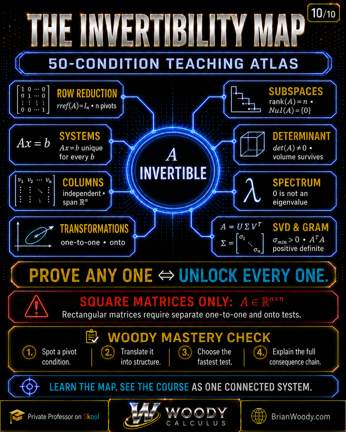
Compress it into six hubs:
- Pivots: \(n\) pivots and \(\operatorname{rref}(A)=I_n\).
- Kernel and image: \(\operatorname{Nul}(A)=\{0\}\) and \(\operatorname{Col}(A)=\mathbb R^n\).
- Systems and maps: exactly one solution for every \(b\); one-to-one and onto.
- Determinant and spectrum: \(\det(A)\ne0\); zero is not an eigenvalue.
- SVD and Gram matrix: \(\sigma_{min}>0\); \(A^TA\) is positive definite.
- Geometry: no independent direction or positive-dimensional volume is collapsed.
If you can prove the bridges among those six hubs, every numbered formulation becomes a definition, a vocabulary translation, or a short corollary.
Part IV — Inverse, Row Reduction, Pivots, and Elementary Matrices
![Exact row reduction of A equals [[2,1],[1,1]] to the identity matrix and B equals [[2,4],[1,2]] to a matrix with a zero row, contrasting full pivots with a missing pivot.](https://k3p6r8v3.delivery.rocketcdn.me/wp-content/uploads/2026/08/Invertible_Matrix_Theorem_Slide_03.png "Row Reduction and Pivots — The Computational Engine of Invertibility")
Conditions 1–6: the computational engine
An inverse \(A^{-1}\) satisfies
A^{-1}A=AA^{-1}=I_n.
\]
Row operations are reversible. If elimination carries \(A\) to \(I_n\), then the product of the corresponding elementary matrices \(E_k\cdots E_1\) satisfies
E_k\cdots E_1A=I_n.
\]
Therefore \(A^{-1}=E_k\cdots E_1\). Conversely, if elimination stops with a missing pivot, the reduced matrix cannot be \(I_n\), so \(A\) cannot have a two-sided inverse.
For an \(n\times n\) matrix, the following are the same event:
A\sim I_n
\iff \operatorname{rref}(A)=I_n
\iff n\text{ pivots}
\iff \text{pivot in every row and column}.
\]
The augmented-matrix inverse algorithm
Row reducing
[A\mid I_n]
\]
performs the same reversible operations on both blocks. If the left block reaches \(I_n\), the right block becomes \(A^{-1}\):
[A\mid I_n]\longrightarrow[I_n\mid A^{-1}].
\]
If the left side cannot reach the identity, the inverse does not exist. This algorithm simultaneously tests invertibility and computes the inverse.
Conditions 29–31: left inverse, right inverse, and elementary factorization
For square matrices, \(BA=I_n\) implies \(A\) is injective: if \(Ax=0\), then \(x=BAx=0\). Injectivity implies invertibility, so \(B=A^{-1}\) and automatically \(AB=I_n\). Similarly, a right inverse \(AC=I_n\) forces surjectivity and hence invertibility.
Each row operation equals multiplication by an elementary matrix. Thus \(A\) is invertible exactly when it is a product of elementary matrices. This is more than a construction trick: it says an invertible matrix is built entirely from reversible operations—row swaps, nonzero scalings, and row replacements.
Part V — Null Space, Independence, Spanning, Bases, Rank, and Nullity
![Invertible Matrix Theorem vector-space map showing that n pivots are equivalent to trivial null space, independent columns, columns spanning R n, a column basis, full rank, and zero nullity, with exact vectors a1 equals [2,1] and a2 equals [1,1].](https://k3p6r8v3.delivery.rocketcdn.me/wp-content/uploads/2026/08/Invertible_Matrix_Theorem_Slide_04.png "Null Space, Independence, Span, and Basis — The Central Pivot Bridge")
Conditions 7–10: no free variable means no hidden direction
Write the columns of \(A\) as \(a_1,\ldots,a_n\). The homogeneous equation
Ax=0
\]
is the vector equation
x_1a_1+\cdots+x_na_n=0.
\]
The columns are linearly independent exactly when the only coefficients producing zero are \(x_1=\cdots=x_n=0\). Therefore
Ax=0\text{ only has }x=0
\iff \operatorname{Nul}(A)=\{0\}
\iff \operatorname{nullity}(A)=0
\iff \{a_1,\ldots,a_n\}\text{ is independent}.
\]
Elimination explains the same chain mechanically. A pivot in every column means no free variable. No free variable means only the zero solution in the homogeneous system.
Conditions 11–15: reaching every direction
The equation \(Ax=b\) asks whether \(b\) is a linear combination of the columns. Therefore \(Ax=b\) is consistent for every \(b\in\mathbb R^n\) exactly when
\operatorname{Col}(A)=\mathbb R^n.
\]
That is the same as saying the columns span \(\mathbb R^n\). Because there are exactly \(n\) columns in an \(n\)-dimensional space, an independent list of \(n\) vectors automatically spans, and a spanning list of \(n\) vectors is automatically independent. Hence the columns form a basis.
Rank packages the image dimension into one number:
\operatorname{rank}(A)=\dim\operatorname{Col}(A).
\]
Rank–nullity packages the input-side accounting:
\operatorname{rank}(A)+\operatorname{nullity}(A)=n.
\]
Thus rank \(n\) and nullity zero are two sides of the same dimension equation.
Existence and uniqueness are different ideas
Students often merge them, but the theorem keeps them distinct before joining them:
| Question | Matrix condition | Transformation language |
|---|---|---|
| Does a solution exist for every \(b\)? | \(\operatorname{Col}(A)=\mathbb R^n\) | \(T\) is onto |
| Can two solutions exist for the same \(b\)? | \(\operatorname{Nul}(A)=\{0\}\) | \(T\) is one-to-one |
| Is there exactly one solution for every \(b\)? | Both conditions hold | \(T\) is bijective |
The difference of any two solutions lies in the null space. If \(Ax_1=b\) and \(Ax_2=b\), then
A(x_1-x_2)=0.
\]
So uniqueness for every consistent system is exactly the statement that the null space is trivial.
Part VI — Systems and Linear Transformations
![Invertible Matrix Theorem systems map separating existence from uniqueness and solving A x equals b for A equals [[2,1],[1,1]] and b equals [5,3], giving the unique solution x equals [2,1].](https://k3p6r8v3.delivery.rocketcdn.me/wp-content/uploads/2026/08/Invertible_Matrix_Theorem_Slide_05.png "Linear Systems — Existence, Uniqueness, and the Solution A Inverse b")
Conditions 23–28: translate equations into maps
The matrix equation \(Ax=b\) and the transformation equation \(T(x)=b\) are the same statement. Consequently:
- \(Ax=b\) is consistent for every \(b\) iff \(T\) is onto.
- \(Ax=b\) has at most one solution for every \(b\) iff \(T\) is one-to-one.
- \(Ax=b\) has exactly one solution for every \(b\) iff \(T\) is bijective.
- \(T\) is bijective iff an inverse transformation \(T^{-1}\) exists.
When \(T(x)=Ax\) is invertible, its inverse is represented by \(A^{-1}\):
T^{-1}(b)=A^{-1}b.
\]
Why one-to-one and onto become equivalent
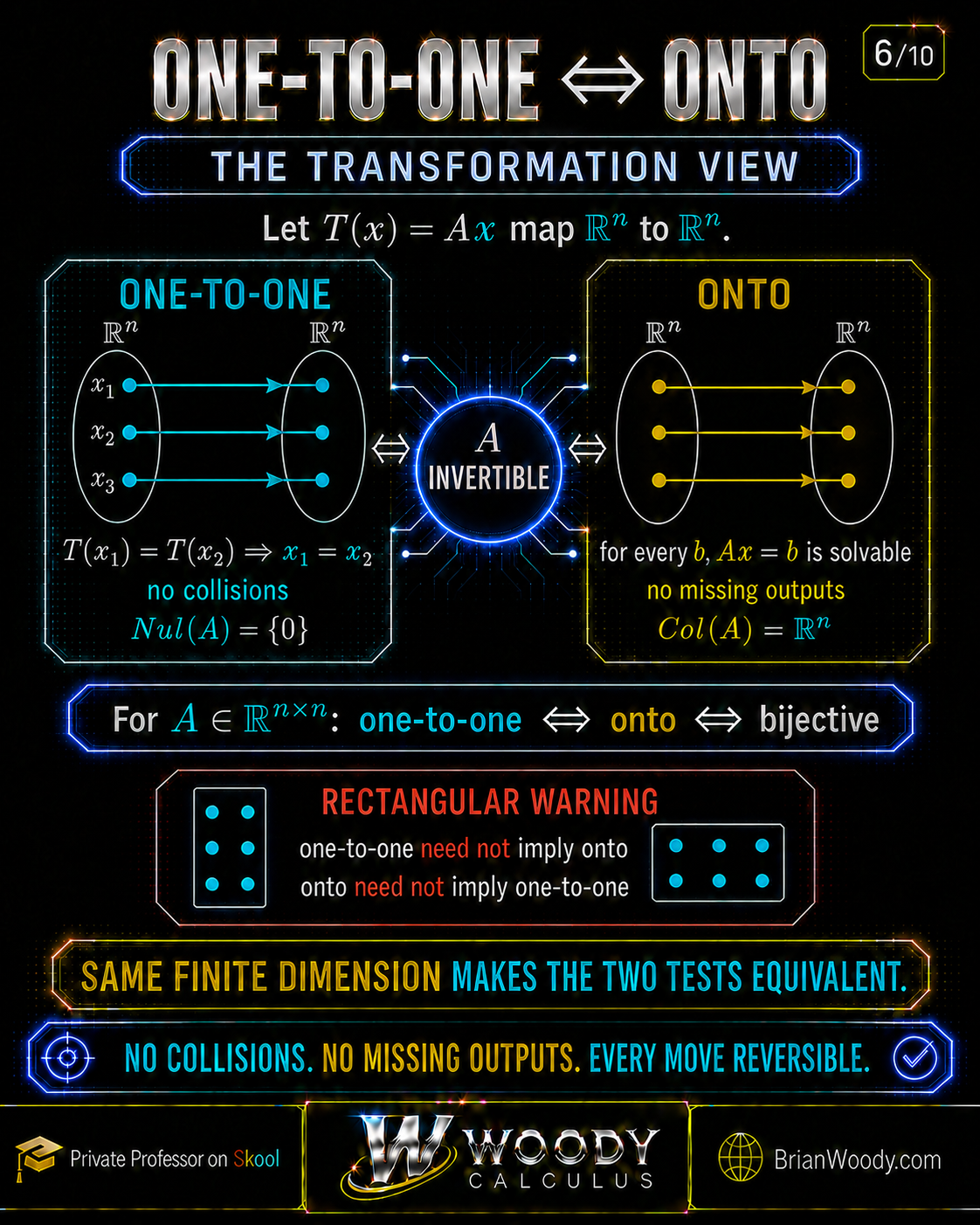
For a general function, injectivity and surjectivity are different. For a rectangular linear map, they are still different. For a linear map from an \(n\)-dimensional space to another \(n\)-dimensional space, rank–nullity forces them together.
If \(T\) is one-to-one, then \(dimker T=0\), so
\dim\operatorname{range}T=n-0=n.
\]
The range is an \(n\)-dimensional subspace of \(\mathbb R^n\), so it must be the entire codomain: \(T\) is onto.
If \(T\) is onto, then the range already has dimension \(n\). Rank–nullity leaves zero dimensions for the kernel, so \(T\) is one-to-one.
The coordinate-change interpretation
A basis matrix \(P=[v_1\ \cdots\ v_n]\) is invertible exactly when its columns form a basis. Then
x=P[x]_{\mathcal B}
\quad\text{and}\quad
[x]_{\mathcal B}=P^{-1}x.
\]
Invertibility is what makes coordinates unique and reversible. If the columns were dependent, one vector could have multiple coordinate lists; if they did not span, some vectors would have no coordinates in that list at all.
Part VII — Determinants, Geometry, Eigenvalues, and Polynomials
![Invertible Matrix Theorem spectral map for A equals [[2,1],[1,1]], showing determinant one, characteristic polynomial t squared minus 3t plus 1, nonzero eigenvalues (3 plus or minus square root 5) over 2, and positive volume scaling.](https://k3p6r8v3.delivery.rocketcdn.me/wp-content/uploads/2026/08/Invertible_Matrix_Theorem_Slide_07.png "Determinants, Eigenvalues, and Polynomial Tests for Invertibility")
Condition 34: the determinant test
The determinant converts the entire theorem into one scalar test:
A\text{ invertible}\iff \det(A)\ne0.
\]
Algebraically, a zero determinant signals dependent rows or columns and a missing pivot. Geometrically, \(|\det(A)|\) is the factor by which \(A\) scales \(n\)-dimensional volume. A nonzero factor means an \(n\)-dimensional region remains \(n\)-dimensional; zero means it collapses into a lower-dimensional set.
The sign of \(\det(A)\) records orientation. A positive determinant preserves orientation, and a negative determinant reverses it. Nonzero alone guarantees invertibility; it does not guarantee orientation preservation.
For a deeper geometric treatment, see Determinants Explained: Algebra, Geometry, and Differential Equations.
Condition 35: zero is not an eigenvalue
By definition, \(\lambda\) is an eigenvalue if there is a nonzero vector \(v\) with
Av=\lambda v.
\]
Setting \(\lambda=0\) gives \(Av=0\) for some \(v\ne0\). Therefore
0\text{ is an eigenvalue}
\iff \operatorname{Nul}(A)\ne\{0\}
\iff A\text{ is singular}.
\]
So an invertible matrix may have positive, negative, real, or complex eigenvalues, but none can equal zero. Invertibility does not imply diagonalizability; a matrix can be invertible and defective.
For the complete spectral foundation, see Eigenvalues and Eigenvectors Explained.
Conditions 36–38: characteristic and minimal polynomials
Using the convention
p_A(t)=\det(tI-A),
\]
we obtain
p_A(0)=\det(-A)=(-1)^n\det(A).
\]
Thus \(p_A(0)\ne0\) exactly when \(\det(A)\ne0\). The sign factor matters in odd dimensions, even though the zero-versus-nonzero test is unchanged.
The minimal polynomial \(m_A\) also detects invertibility. If \(m_A(0)=0\), then \(m_A(t)=tq(t)\), so \(Aq(A)=0\); the minimality structure forces zero into the spectrum. If \(m_A(0)\ne0\), write
m_A(t)=c_0+tq(t),\qquad c_0\ne0.
\]
Since \(m_A(A)=0\),
c_0I+Aq(A)=0
\quad\Longrightarrow\quad
A\left(-\frac{1}{c_0}q(A)\right)=I.
\]
Therefore \(A^{-1}\) is a polynomial in \(A\). Cayley–Hamilton gives a similar construction from the characteristic polynomial.
Part VIII — Rows, Transpose, and the Four Fundamental Subspaces
Conditions 16–22: row–column duality
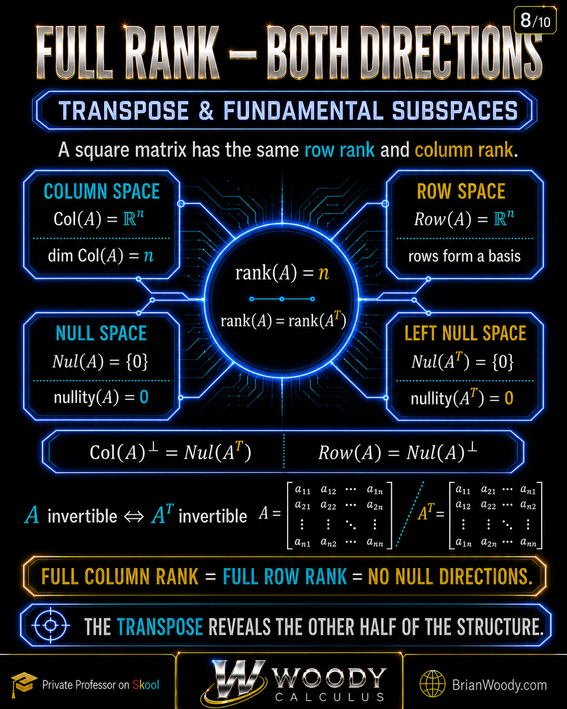
The columns of \(A^T\) are the rows of \(A\). Since
\operatorname{rank}(A)=\operatorname{rank}(A^T),
\]
full column rank for \(A\) is the same as full column rank for \(A^T\). That immediately connects invertibility of \(A\), invertibility of \(A^T\), independent rows, spanning rows, a row basis, and zero transpose nullity.
Also,
(A^{-1})^T=(A^T)^{-1},
\]
because transposing \(AA^{-1}=I\) reverses the product order.
The four fundamental subspaces
For \(A\in\mathbb R^{m\times n}\), the four fundamental subspaces are
- \(\operatorname{Col}(A)\subseteq\mathbb R^m\),
- \(\operatorname{Nul}(A^T)\subseteq\mathbb R^m\),
- \(\operatorname{Row}(A)=\operatorname{Col}(A^T)\subseteq\mathbb R^n\),
- \(\operatorname{Nul}(A)\subseteq\mathbb R^n\).
They pair through orthogonal complements:
\operatorname{Col}(A)^\perp=\operatorname{Nul}(A^T),
\qquad
\operatorname{Row}(A)=\operatorname{Nul}(A)^\perp.
\]
For an invertible \(n\times n\) matrix, both null spaces are zero and both row and column spaces are all of \(\mathbb R^n\). Conditions 32 and 33 are direct restatements of those orthogonal-complement identities.
Why this matters for solvability
For any matrix—not necessarily square—the system \(Ax=b\) is consistent exactly when \(b\in\operatorname{Col}(A)\). Equivalently, \(b\) must be orthogonal to every vector in \(\operatorname{Nul}(A^T)\). This is the finite-dimensional Fredholm alternative:
Ax=b\text{ is solvable}
\iff y^Tb=0\text{ for every }y\text{ with }A^Ty=0.
\]
When \(A\) is invertible, \(\operatorname{Nul}(A^T)=\{0\}\), so there is no compatibility obstruction and every \(b\) is reachable.
Part IX — SVD, Gram Matrices, Lower Bounds, and Conditioning
Conditions 39–40: singular values
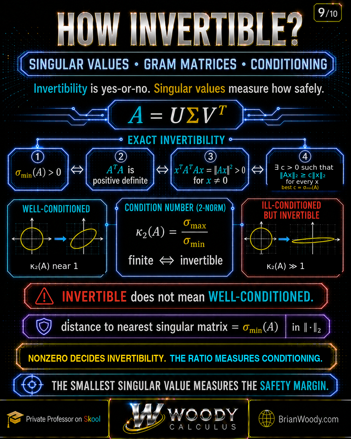
Every real matrix has a singular value decomposition
A=U\Sigma V^T,
\]
where (U) and (V) are orthogonal and the diagonal entries of (Sigma) are the singular values
\sigma_1\ge\sigma_2\ge\cdots\ge\sigma_n\ge0.
\]
Orthogonal factors only rotate or reflect. The singular values measure stretches along perpendicular directions. A zero singular value means one direction is flattened completely. Thus
A\text{ invertible}
\iff \operatorname{rank}(A)=n
\iff \sigma_n=\sigma_{\min}(A)>0.
\]
Conditions 41–44: the Gram matrix
The Gram matrix is \(A^TA\). Its central identity is
x^TA^TAx=(Ax)^T(Ax)=\|Ax\|_2^2.
\]
Therefore \(x^TA^TAx>0\) for every \(x\ne0\) exactly when \(Ax\ne0\) for every \(x\ne0\). That is injectivity, which is invertibility for a square matrix. Hence
A\text{ invertible}
\iff A^TA\text{ invertible}
\iff A^TA\text{ positive definite}.
\]
The eigenvalues of \(A^TA\) are \(\sigma_i^2\). Consequently the Gram determinant satisfies
\det(A^TA)=\det(A)^2=\prod_{i=1}^n\sigma_i^2.
\]
It is positive exactly when no singular value is zero.
Condition 45: bounded below
The correct equivalent statement is:
\exists c>0\text{ such that }\|Ax\|_2\ge c\|x\|_2
\quad\text{for every }x.
\]
This says that \(A\) cannot shrink any nonzero input arbitrarily close to zero relative to its size. The best possible constant is \(c=\sigma_{\min}(A)\).
Be careful: the inequality \(\|Ax\|_2\ge\sigma_{\min}(A)\|x\|_2\) is true for every matrix. It becomes an invertibility test only when the lower-bound constant is required to be strictly positive.
Condition 46: condition number
The spectral condition number is
\kappa_2(A)=\|A\|_2\|A^{-1}\|_2
=\frac{\sigma_{\max}(A)}{\sigma_{\min}(A)}.
\]
It is finite exactly when \(A\) is invertible. But “finite” can still mean enormous. A large condition number signals that relative errors in data or rounding can be strongly amplified.
Critical distinction: nonzero \(\sigma_{\min}\) decides exact invertibility. The ratio \(\sigma_{\max}/\sigma_{\min}\) measures conditioning. The scale-dependent statement “\(\sigma_{\min}\) is small” does not by itself mean ill-conditioned; \(10^{-6}I\) has a small smallest singular value but \(\kappa_2=1\).
In spectral norm, the distance from \(A\) to the nearest singular matrix equals \(\sigma_{\min}(A)\). This explains why the smallest singular value is a safety margin while the condition number is a relative sensitivity measure.
Part X — Complete Worked Examples
Invertible example: activate the whole theorem
Let
A=\begin{bmatrix}2&1\\1&1\end{bmatrix}.
\]
Its determinant is
\det(A)=2(1)-1(1)=1\ne0.
\]
That single calculation is enough to invoke all fifty conditions. To see the connections rather than merely cite them, row reduce:
\begin{bmatrix}2&1\\1&1\end{bmatrix}
\xrightarrow{R_1\leftrightarrow R_2}
\begin{bmatrix}1&1\\2&1\end{bmatrix}
\xrightarrow{R_2-2R_1}
\begin{bmatrix}1&1\\0&-1\end{bmatrix}
\longrightarrow I_2.
\]
There are two pivots and no free variables. Therefore the columns are independent. Because there are two independent columns in \(\mathbb R^2\), they form a basis and span the plane. The null space is \(\{0\}\), rank is two, nullity is zero, and the associated map is one-to-one and onto.
The inverse is
A^{-1}=\begin{bmatrix}1&-1\\-1&2\end{bmatrix}.
\]
For \(b=[5,3]^T\),
x=A^{-1}b
=\begin{bmatrix}1&-1\\-1&2\end{bmatrix}
\begin{bmatrix}5\\3\end{bmatrix}
=\begin{bmatrix}2\\1\end{bmatrix},
\]
and \(Ax=[5,3]^T\) verifies the answer.
Its characteristic polynomial is
p_A(t)=\det(tI-A)=t^2-3t+1,
\]
with eigenvalues
\lambda_{1,2}=\frac{3\pm\sqrt5}{2}.
\]
Both are nonzero. Because this particular \(A\) is symmetric positive definite, its singular values equal its positive eigenvalues: approximately \(2.618\) and \(0.382\). Thus
\kappa_2(A)\approx\frac{2.618}{0.382}\approx6.854.
\]
Also,
A^TA=\begin{bmatrix}5&3\\3&2\end{bmatrix},
\qquad \det(A^TA)=1>0,
\]
and the unit square maps to a parallelogram of area \(|\det A|=1\).
Singular example: collapse the whole theorem
Now let
B=\begin{bmatrix}2&4\\1&2\end{bmatrix}.
\]
Its determinant is zero and its second column is twice its first. Row reduction gives
\operatorname{rref}(B)=\begin{bmatrix}1&2\\0&0\end{bmatrix}.
\]
There is one pivot and one free variable. Indeed,
B\begin{bmatrix}-2\\1\end{bmatrix}=0.
\]
So the null space is nontrivial, the columns are dependent, rank is one, nullity is one, and the map is not one-to-one. Its column space is only a line, so the map is not onto \(\mathbb R^2\). Some right-hand sides have no solution, while consistent systems have infinitely many solutions.
Zero is an eigenvalue and singular value. The unit square collapses to a line segment with area zero. No inverse exists. Again, one decisive failure reveals the entire world.
Side-by-side ledger
| Feature | Invertible \(A\) | Singular \(B\) |
|---|---|---|
| RREF | \(I_2\) | \(left[\begin{smallmatrix}1&2\\0&0\end{smallmatrix}\right]\) |
| Rank / nullity | \(2/0\) | \(1/1\) |
| Homogeneous system | Only \(x=0\) | Nonzero solutions |
| Columns | Basis of \(\mathbb R^2\) | Dependent; span a line |
| \(Ax=b\) | One solution for every \(b\) | None or infinitely many |
| Transformation | One-to-one and onto | Neither |
| Determinant | \(1\) | \(0\) |
| Zero eigenvalue? | No | Yes |
| Smallest singular value | Positive | Zero |
| Geometry | Plane stays two-dimensional | Plane collapses to a line |
Part XI — The Proof Network
Proof spine 1: elimination
A\text{ invertible}
\iff A\sim I_n
\iff \operatorname{rref}(A)=I_n
\iff A\text{ has }n\text{ pivots}.
\]
Reversible row operations provide both directions and give the elementary-matrix factorization.
Proof spine 2: pivots to kernel and image
n\text{ pivots}
\iff \text{no free variables}
\iff \operatorname{Nul}(A)=\{0\}
\iff \text{columns independent}.
\]
The same \(n\) pivots include a pivot in every row:
n\text{ pivots}
\iff \operatorname{Col}(A)=\mathbb R^n
\iff \text{columns span }\mathbb R^n.
\]
Rank–nullity and the basis theorem attach rank, nullity, and basis language.
Proof spine 3: systems and transformations
\operatorname{Nul}(A)=\{0\}
\iff T\text{ is one-to-one},
\]
while
\operatorname{Col}(A)=\mathbb R^n
\iff T\text{ is onto}
\iff Ax=b\text{ is consistent for every }b.
\]
The square equal-dimension hypothesis turns one-to-one into onto and combines existence with uniqueness.
Proof spine 4: determinant and spectrum
Elimination or the adjugate identity establishes
\det(A)\ne0\iff A^{-1}\text{ exists}.
\]
The eigenvalue definition establishes
0\in\sigma(A)
\iff \exists x\ne0:Ax=0
\iff A\text{ singular}.
\]
Evaluating \(p_A(t)=\det(tI-A)\) at zero and using Cayley–Hamilton attaches the polynomial conditions.
Proof spine 5: transpose and subspaces
Rank is unchanged by transpose, so full row rank and full column rank coincide. The identities
\operatorname{Col}(A)^\perp=\operatorname{Nul}(A^T),
\qquad
\operatorname{Row}(A)=\operatorname{Nul}(A)^\perp
\]
attach the orthogonality conditions.
Proof spine 6: SVD and Gram matrices
From
x^TA^TAx=\|Ax\|_2^2,
\]
positive definiteness of \(A^TA\) is exactly triviality of the kernel. The eigenvalues of \(A^TA\) are \(\sigma_i^2\), so positive definiteness, positive singular values, a positive lower bound, and finite \(\kappa_2\) meet at \(\sigma_{\min}>0\).
Proof spine 7: geometry and dimension
The transformed unit cube has volume \(|\det A|\), so positive volume equals nonzero determinant. An injective linear map preserves independent sets and the dimension of every subspace. Conversely, if every one-dimensional subspace keeps dimension one, no nonzero vector can map to zero, so the kernel is trivial.
A short circular proof worth memorizing
If your instructor requests a compact proof of the classical core, use this loop:
\operatorname{rref}(A)=I_n
\Rightarrow \operatorname{Nul}(A)=\{0\}
\Rightarrow T\text{ one-to-one}
\Rightarrow T\text{ onto}
\Rightarrow \operatorname{Col}(A)=\mathbb R^n
\Rightarrow n\text{ pivots}
\Rightarrow \operatorname{rref}(A)=I_n.
\]
Then attach the inverse, determinant, basis, rank, spectrum, transpose, and SVD families through their defining bridge identities.
Part XII — Fastest Tests, Applications, Mistakes, and Mastery
Which invertibility test should you use?
| Information already available | Fastest test | Why |
|---|---|---|
| Small numerical matrix | Row reduce or compute \(\det(A)\) | Direct and decisive |
| Matrix is triangular | Check diagonal entries | \(\det(A)\) is their product; pivots are visible |
| Homogeneous system is solved | Check for free variables | Only the trivial solution means invertible |
| Columns described geometrically | Test independence or spanning | Either is enough for \(n\) vectors in \(\mathbb R^n\) |
| Eigenvalues known | Check whether any \(\lambda_i=0\) | Zero eigenvalue is exactly singularity |
| SVD known | Check \(\sigma_{\min}>0\) | Also reveals numerical safety margin |
| \(A^TA\) appears | Test positive definiteness | \(x^TA^TAx=\|Ax\|^2\) |
| Linear map language | Test kernel or range | Trivial kernel / full range |
| Product \(A=BC\) | Use product rules | A product is invertible iff both square factors are invertible |
| Numerical computation | Use rank-revealing QR or SVD | More reliable than explicit inverse or raw determinant |
In numerical software, avoid deciding near-singularity from exact equality with a floating-point determinant. Rank-revealing factorizations and singular values are safer because they expose scale and sensitivity.
Applications across linear algebra and beyond
Coordinate changes. A change-of-basis matrix must be invertible so coordinates can move both directions without ambiguity.
Differential equations. For \(x^{\prime}=Ax\), an invertible \(A\) means zero is not an eigenvalue, so the origin has no center direction caused by a zero eigenvalue. Stability still depends on the real parts of all eigenvalues, not invertibility alone. See Phase Portraits, Eigenvalues, and Stability.
Least squares. If a rectangular design matrix \(X\) has independent columns, \(X^TX\) is invertible and the normal equations have the unique solution
\hat\beta=(X^TX)^{-1}X^Ty.
\]
Notice the distinction: \(X\) itself need not be square; invertibility is asserted for the square Gram matrix \(X^TX\).
Eigenvector matrices. A matrix \(P\) of eigenvectors is invertible exactly when those eigenvectors form a basis. Then \(A=PDP^{-1}\). An invertible \(A\) need not be diagonalizable; these are separate properties.
Numerical linear algebra. Solving \(Ax=b\) depends not only on whether \(A^{-1}\) exists in exact arithmetic but also on conditioning. A huge \(\kappa(A)\) can make computed solutions sensitive to small perturbations.
Information and data transformations. An invertible linear layer has no collisions: each output comes from exactly one input. Rank deficiency means dimensional information is destroyed.
Advanced equivalent corollaries
The following are useful extensions rather than part of the headline count:
- \(A^k\) is invertible for some positive integer \(k\), equivalently for every positive integer \(k\).
- For every \(D\in M_n(\mathbb R)\), \(AX=D\) has exactly one solution \(X\).
- For every \(D\in M_n(\mathbb R)\), \(XA=D\) has exactly one solution \(X\).
- Left multiplication \(X\mapsto AX\) and right multiplication \(X\mapsto XA\) are invertible operators on \(M_n(\mathbb R)\).
- Matrix cancellation by \(A\) is valid on both sides.
- For \(n\ge2\), \(\operatorname{adj}(A)\) is invertible.
- \(A\) lies a positive spectral-norm distance from the singular matrices, equal to \(\sigma_{\min}(A)\).
- The reciprocal condition number is positive.
These examples also prove why no final universal count exists.
Common mistakes and exam traps
- Forgetting the square hypothesis. One-to-one does not imply onto for a tall matrix, and onto does not imply one-to-one for a wide matrix.
- Saying “the determinant exists, so the matrix is invertible.” Every square matrix has a determinant; it must be nonzero.
- Confusing “consistent” with “unique.” Existence is controlled by the column space; uniqueness is controlled by the null space.
- Checking only rows or only columns without using squareness. Pivot-every-row and pivot-every-column coincide only in the square full-rank case.
- Believing nonzero eigenvalues imply diagonalizability. They imply invertibility, not a complete eigenbasis.
- Believing invertible means numerically safe. A matrix can have a positive but tiny relative safety margin and a huge condition number.
- Using \(A^T\) instead of \(A^*\) over \(\mathbb C\). Inner-product and Gram statements require conjugation.
- Computing \(A^{-1}\) when only a solution is needed. Solve \(Ax=b\) by factorization; explicitly forming the inverse is usually slower and less stable.
- Treating a one-sided inverse of a rectangular matrix as two-sided. Dimensions and rank determine which side can exist.
- Dropping the sign convention in the characteristic polynomial. For \(p_A(t)=\det(tI-A)\), \(p_A(0)=(-1)^n\det(A)\).
The Woody mastery method
Do not memorize fifty isolated sentences. Practice translation from one dialect to another:
- Start with one condition, such as “\(Ax=0\) has only the trivial solution.”
- Translate it into kernel language: \(\operatorname{Nul}(A)=\{0\}\).
- Translate kernel into columns: the columns are independent.
- Use squareness: \(n\) independent columns in \(\mathbb R^n\) form a basis and span.
- Translate span into systems and maps: every \(b\) is reachable, so \(T\) is onto.
- Return to computation: full span means a pivot in every row; square size gives \(n\) pivots and RREF \(I_n\).
- Attach determinant, eigenvalue, SVD, and geometry tests.
Your goal is to rebuild the network from any starting point. If you can explain three different routes from a given condition to invertibility, you understand the theorem rather than merely recognizing its wording.
Part XIII — Linear Algebra Reference Dictionary
This dictionary makes the lesson self-contained for a student meeting some of the vocabulary for the first time. Each entry gives a definition, its place in the theorem, and the fastest bridge to invertibility.
Inverse matrix
An inverse of a square matrix \(A\) is a matrix \(A^{-1}\) satisfying
AA^{-1}=A^{-1}A=I_n.
\]
Multiplying by \(A\) performs a reversible linear transformation; multiplying by \(A^{-1}\) reverses it. The inverse is unique. If \(B\) and \(C\) were both inverses, then
B=BI_n=B(AC)=(BA)C=I_nC=C.
\]
Useful rules include
(AB)^{-1}=B^{-1}A^{-1},\qquad
(A^T)^{-1}=(A^{-1})^T,\qquad
(A^k)^{-1}=(A^{-1})^k.
\]
The reverse order in the product rule matters because matrix multiplication is generally not commutative.
Row echelon form, reduced row-echelon form, and pivots
A matrix is in row echelon form when nonzero rows appear above zero rows, each leading entry moves right as you move down, and entries below each leading entry are zero. Reduced row-echelon form adds two conditions: each leading entry is \(1\), and it is the only nonzero entry in its column.
A pivot position is the location of a leading entry in an echelon form. Pivots reveal rank and identify basic variables. Columns without pivots correspond to free variables in \(Ax=0\). For a square matrix, no free variables means a pivot in every column; \(n\) pivots then also means a pivot in every row.
Homogeneous and nonhomogeneous systems
A system \(Ax=0\) is homogeneous and is always consistent because \(x=0\) is a solution. Its decisive question is uniqueness: are there nonzero solutions? Those nonzero solutions are precisely the information-losing directions of \(A\).
A system \(Ax=b\) is nonhomogeneous when \(b\ne0\). Its decisive questions are existence and uniqueness. Existence asks whether \(b\) lies in the column space. Uniqueness asks whether the homogeneous system has only the zero solution.
If \(x_p\) is one particular solution, every solution has the form
x=x_p+x_h,\qquad x_h\in\operatorname{Nul}(A).
\]
This formula explains the three standard possibilities: no solution, exactly one solution, or infinitely many solutions. For an invertible coefficient matrix, only the exactly-one case occurs, for every \(b\).
Null space or kernel
The null space is
\operatorname{Nul}(A)=\{x\in\mathbb R^n:Ax=0\}.
\]
It records every direction erased by the transformation. A trivial null space means no nonzero vector is erased, so the map is one-to-one. A nontrivial null space gives a collision: if \(Az=0\) with \(z\ne0\), then \(A(x+z)=Ax\).
Column space or range
The column space is
\operatorname{Col}(A)=\{Ax:x\in\mathbb R^n\}.
\]
It is the set of all reachable outputs and also the span of the columns. The system \(Ax=b\) is solvable precisely when \(b\in\operatorname{Col}(A)\). For a square invertible matrix, the column space is all of \(\mathbb R^n\).
Linear independence
Vectors \(v_1,\ldots,v_k\) are linearly independent if
c_1v_1+\cdots+c_kv_k=0
\]
forces \(c_1=\cdots=c_k=0\). Applied to the columns of \(A\), that equation is \(Ax=0\). Column independence and a trivial null space are therefore exactly the same statement written in two dialects.
Span
The span of a list of vectors is the set of all their linear combinations. The columns of \(A\) span \(\mathbb R^n\) when every \(b\in\mathbb R^n\) can be expressed as
b=x_1a_1+\cdots+x_na_n=Ax.
\]
Thus spanning columns, universal consistency of \(Ax=b\), full column space, and onto behavior are the same fact.
Basis and coordinates
A basis is a linearly independent spanning set. Independence gives unique coordinates; spanning guarantees that coordinates exist. A square matrix is invertible precisely when its columns form a basis of \(\mathbb R^n\). The inverse converts standard coordinates back into coordinates relative to that basis.
The basis theorem is a key finite-dimensional shortcut: every independent list of \(n\) vectors in \(\mathbb R^n\) is automatically a basis, and every spanning list of \(n\) vectors is automatically a basis.
Rank and nullity
Rank is the dimension of the image:
\operatorname{rank}(A)=\dim\operatorname{Col}(A).
\]
Nullity is the dimension of the kernel:
\operatorname{nullity}(A)=\dim\operatorname{Nul}(A).
\]
For a matrix with \(n\) columns, rank–nullity says
\operatorname{rank}(A)+\operatorname{nullity}(A)=n.
\]
Invertibility is the extreme full-information case: rank \(n\) and nullity \(0\).
One-to-one, onto, and bijective
A map is one-to-one if different inputs always produce different outputs. For a linear map, this is equivalent to a trivial kernel.
A map is onto if every target in the codomain is reached. For a matrix map, this is equivalent to the column space equaling the codomain.
A map is bijective if it is both one-to-one and onto. Bijectivity is the function-level definition of invertibility. The special square finite-dimensional fact is that either one-to-one or onto alone forces the other.
Determinant
The determinant is a signed volume-scaling factor. It is multilinear in the rows or columns, changes sign when two rows are swapped, and vanishes when rows or columns are dependent. Its multiplication rule,
\det(AB)=\det(A)\det(B),
\]
immediately shows that if \(A\) is invertible, then
1=\det(I)=\det(A)\det(A^{-1}),
\]
so \(\det(A)\ne0\) and \(\det(A^{-1})=1/\det(A)\).
Eigenvalue and spectrum
An eigenvalue \(\lambda\) is a scalar for which \(Av=\lambda v\) for some nonzero eigenvector \(v\). The spectrum is the set of eigenvalues, counted with context-appropriate multiplicity. The only eigenvalue that decides invertibility by itself is zero:
0\notin\sigma(A)\iff A\text{ is invertible}.
\]
Other spectral properties answer different questions. For example, diagonalizability asks whether there are enough independent eigenvectors, while stability of \(x^{\prime}=Ax\) depends on the real parts of eigenvalues.
Singular value
The singular values are the nonnegative square roots of the eigenvalues of \(A^TA\). Unlike eigenvalues, they are always real and nonnegative. They measure the principal stretch factors of the transformation. Rank equals the number of positive singular values, and invertibility requires all \(n\) to be positive.
Gram matrix and positive definiteness
The Gram matrix \(A^TA\) stores all column inner products. Its \((i,j)\) entry is \(a_i^Ta_j\). It is always symmetric and positive semidefinite because
x^TA^TAx=\|Ax\|_2^2\ge0.
\]
It is positive definite precisely when equality can occur only at \(x=0\), which is precisely when the columns of \(A\) are independent.
Condition number
The condition number estimates relative sensitivity. In the Euclidean norm,
\kappa_2(A)=\frac{\sigma_{\max}(A)}{\sigma_{\min}(A)}.
\]
An orthogonal matrix has condition number \(1\), the best possible value. A singular matrix has infinite condition number under the standard convention. An invertible matrix with a very large condition number is mathematically reversible but numerically delicate.
Part XIV — Implication Recipes and Solved Practice
These examples demonstrate how to use the theorem efficiently. Each solution names the shortest bridge and then unlocks the requested conclusion.
Recipe 1: from a homogeneous system to every right-hand side
Given: \(A\in\mathbb R^{n\times n}\) and \(Ax=0\) has only \(x=0\).
Prove: \(Ax=b\) has exactly one solution for every \(b\in\mathbb R^n\).
The given condition says \(\operatorname{Nul}(A)=\{0\}\), so \(A\) is one-to-one. Because the map is square and finite-dimensional, one-to-one implies onto. Onto gives existence for every \(b\), and the trivial kernel gives uniqueness. Therefore every system has exactly one solution.
Recipe 2: from spanning rows to a nonzero determinant
Given: the rows of \(A\in\mathbb R^{n\times n}\) span \(\mathbb R^n\).
Prove: \(\det(A)\ne0\).
Spanning rows give \(\operatorname{Row}(A)=\mathbb R^n\), so row rank is \(n\). Row rank equals column rank, hence \(\operatorname{rank}(A)=n\). Full rank is equivalent to invertibility, and an invertible matrix has nonzero determinant.
Recipe 3: from a left inverse to unique solvability
Given: \(BA=I_n\).
Prove: \(Ax=b\) has exactly one solution for every \(b\).
If \(Ax=0\), multiply by \(B\):
x=I_nx=BAx=0.
\]
Thus \(A\) has trivial kernel and is injective. Since \(A\) is square, it is invertible. In fact \(B=A^{-1}\), so the unique solution is \(x=Bb\).
Recipe 4: from a Gram matrix to independent columns
Given: \(A^TA\) is positive definite.
Prove: the columns of \(A\) are linearly independent.
If \(Ax=0\), then
x^TA^TAx=\|Ax\|_2^2=0.
\]
Positive definiteness allows equality only for \(x=0\). Therefore the null space is trivial, which is exactly column independence.
Recipe 5: from a singular value to volume
Given: \(\sigma_{\min}(A)>0\).
Prove: the image of the unit cube has positive volume.
Positive smallest singular value means every singular value is positive, so their product is positive. Since
|\det(A)|=\prod_{i=1}^n\sigma_i,
\]
the determinant is nonzero. The transformed unit cube therefore has positive \(n\)-dimensional volume.
Recipe 6: if a power is invertible
Given: \(A^k\) is invertible for some positive integer \(k\).
Prove: \(A\) is invertible.
Determinants provide the shortest route:
\det(A^k)=\det(A)^k.
\]
The left side is nonzero, so \(\det(A)\ne0\). Alternatively, if \(Ax=0\), then \(A^kx=0\); invertibility of \(A^k\) forces \(x=0\), so \(A\) has trivial kernel.
Recipe 7: if a product is invertible
Given: \(A,B\in\mathbb R^{n\times n}\) and \(AB\) is invertible.
Prove: both \(A\) and \(B\) are invertible.
Using determinants,
0\ne\det(AB)=\det(A)\det(B),
\]
so neither factor can have zero determinant. Thus both are invertible. The inverse is
(AB)^{-1}=B^{-1}A^{-1}.
\]
This conclusion requires square factors of the same size. Rectangular factorization needs a more careful rank argument.
Recipe 8: parameter values that make a matrix invertible
Determine when
A(k)=\begin{bmatrix}k&2\\3&k-1\end{bmatrix}
\]
is invertible. Compute
\det A(k)=k(k-1)-6=k^2-k-6=(k-3)(k+2).
\]
Therefore \(A(k)\) is invertible for every real \(k\) except
k=3\quad\text{and}\quad k=-2.
\]
At either excluded value, the determinant is zero, rank drops, a nonzero null vector appears, zero becomes an eigenvalue, and all other IMT conditions fail.
Recipe 9: a triangular matrix
For an upper triangular matrix,
U=\begin{bmatrix}
u_{11}&*&\cdots&*\\
0&u_{22}&\cdots&*\\
\vdots&\ddots&\ddots&\vdots\\
0&\cdots&0&u_{nn}
\end{bmatrix},
\]
the determinant is the product of diagonal entries:
\det(U)=u_{11}u_{22}\cdots u_{nn}.
\]
Therefore \(U\) is invertible exactly when every diagonal entry is nonzero. Those diagonal entries are also the eigenvalues, and they occupy the pivot positions. One visual check simultaneously reads the elimination, determinant, and spectrum conditions.
Recipe 10: invertible but ill-conditioned
Let
C_\varepsilon=\begin{bmatrix}1&0\\0&\varepsilon\end{bmatrix},
\qquad 0<\varepsilon\ll1.
\]
Then \(\det(C_\varepsilon)=\varepsilon\ne0\), so the matrix is invertible. Its singular values are \(1\) and \(\varepsilon\), giving
\kappa_2(C_\varepsilon)=\frac1\varepsilon.
\]
As \(\varepsilon\) approaches zero, exact invertibility remains true for every positive \(\varepsilon\), but numerical sensitivity becomes arbitrarily severe. This is the cleanest example of why “invertible” and “well-conditioned” are not synonyms.
Recipe 11: a rectangular Gram matrix
Let \(X\in\mathbb R^{m\times n}\) with \(m\ge n\). Then
X^TX\text{ is invertible}
\iff \operatorname{Nul}(X)=\{0\}
\iff \text{the columns of }X\text{ are independent}.
\]
The proof uses
z^TX^TXz=\|Xz\|_2^2.
\]
This is not the square IMT applied directly to \(X\); it is the IMT applied to the square \(n\times n\) Gram matrix \(X^TX\), together with a kernel identity. This distinction is central in least squares and statistics.
Recipe 12: cancellation
Suppose \(A\) is invertible and \(AB=AC\). Multiplying on the left by \(A^{-1}\) gives
B=C.
\]
If instead \(BA=CA\), multiply on the right by \(A^{-1}\). Cancellation works because \(A\) is invertible. It is not valid for arbitrary matrices: a singular matrix can erase the nonzero difference \(B-C\).
Self-check problems
Try each problem using only one or two implication bridges before reading the answer.
-
If \(\operatorname{nullity}(A^T)=0\) for a square matrix, what can you conclude about the rows, determinant, and every system \(Ax=b\)?
Answer: \(A^T\) is injective and invertible; the rows of \(A\) form a basis, \(\det(A)\ne0\), and every \(Ax=b\) has exactly one solution. -
If the columns of \(A\) span \(\mathbb R^n\), can zero be an eigenvalue?
Answer: No. Spanning gives full rank and invertibility, so the null space is trivial and zero is absent from the spectrum. -
If \(\det(A^TA)=0\), what happens to \(\sigma_{\min}(A)\)?
Answer: Since \(\det(A^TA)=\prod_i\sigma_i^2\), at least one singular value is zero; in particular \(\sigma_{\min}(A)=0\), so \(A\) is singular. -
If an \(n\times n\) matrix maps one basis to a basis, must it be invertible?
Answer: Yes. The images of that basis span the codomain and are independent, so the transformation is bijective. Condition 48 uses “every basis,” but even one mapped basis is enough. -
If \(A\) is invertible, is \(A+A^T\) necessarily invertible?
Answer: No. Take \(A=\left[\begin{smallmatrix}0&-1\\1&0\end{smallmatrix}\right]\). Then \(A\) is invertible but \(A+A^T=0\). Invertibility is not preserved by matrix addition.
Invertible Matrix Theorem FAQ
What does the Invertible Matrix Theorem say?
For a square matrix, many conditions are equivalent: having an inverse, reducing to the identity, having full pivots and rank, having a trivial null space, having columns that form a basis, solving Ax = b uniquely for every b, defining a bijection, having nonzero determinant, having no zero eigenvalue, and having positive singular values.
Why is the Invertible Matrix Theorem important?
It is the central connection map of introductory linear algebra. It lets one inexpensive test answer questions about systems, vector spaces, transformations, determinants, eigenvalues, geometry, and numerical behavior.
How many conditions are in the Invertible Matrix Theorem?
There is no universal final count because authors split and combine equivalent formulations differently. MathWorld gives 23 numbered classical conditions; this Woody Calculus atlas organizes 50 useful formulations and states its counting rule explicitly.
Does the Invertible Matrix Theorem apply only to square matrices?
The full all-or-nothing theorem does. Rectangular matrices have related full-row-rank and full-column-rank theorems, but one-to-one and onto are not equivalent and left and right inverses need not coincide.
What is the difference between invertible and nonsingular?
There is no difference in this setting. An invertible matrix is also called nonsingular; a matrix without an inverse is singular.
How can you tell whether a matrix is invertible?
For a square matrix, test any equivalent condition: row reduce to I, find n pivots, show det(A) is nonzero, show Ax = 0 has only x = 0, show rank n, check that zero is not an eigenvalue, or verify σ_min is positive.
What is the fastest invertibility test?
It depends on the information supplied. Use diagonal entries for triangular matrices, a determinant for small exact matrices, free variables after elimination, known eigenvalues, or the smallest singular value in numerical work.
Why does RREF equal to the identity imply invertibility?
Row operations are reversible and correspond to multiplication by invertible elementary matrices. If elimination carries A to I, reversing those operations carries I back to A and constructs A inverse.
Why does a pivot in every column imply invertibility?
A pivot in every column means there are no free variables, so Ax = 0 has only the trivial solution. For a square matrix, that gives n pivots, including a pivot in every row, and therefore invertibility.
Why does a pivot in every row imply invertibility?
A pivot in every row makes the columns span R n. A square n by n matrix then has n pivots, so it also has a pivot in every column and is invertible.
Why does a trivial null space imply invertibility?
Nul(A) = {0} means the associated map is one-to-one. A one-to-one linear map from R n to R n has rank n by rank-nullity, so it is onto and invertible.
Why do linearly independent columns imply the columns span R n?
A square n by n matrix has exactly n columns. Any linearly independent list of n vectors in the n-dimensional space R n is automatically a basis and therefore spans R n.
Why does spanning imply linear independence for a square matrix?
Any spanning list of exactly n vectors in an n-dimensional space is a basis. A basis is linearly independent. This conclusion can fail when the list contains more than n vectors.
How are rank and nullity connected to invertibility?
Rank-nullity gives rank(A) + nullity(A) = n. Invertibility is equivalent to rank n and therefore nullity zero.
Why does Ax = b have exactly one solution when A is invertible?
Multiplying Ax = b by A inverse gives x = A inverse b, which proves existence. If two solutions existed, their difference would lie in Nul(A), which is trivial, proving uniqueness.
Can an invertible system have no solution or infinitely many solutions?
No. If the square coefficient matrix is invertible, Ax = b has exactly one solution for every b. No-solution and infinitely-many-solution cases require a singular coefficient matrix.
Why are one-to-one and onto equivalent for square matrices?
For T from R n to R n, rank-nullity says dimension of the kernel plus dimension of the range equals n. A zero-dimensional kernel forces an n-dimensional range, and an n-dimensional range forces a zero-dimensional kernel.
Does one-to-one imply onto for a rectangular matrix?
Not generally. A tall matrix can define a one-to-one map into a higher-dimensional codomain without reaching every output. A wide matrix can be onto while having a nontrivial kernel.
Does a left inverse imply a right inverse?
For a square matrix, yes: either one-sided inverse forces full rank and is the unique two-sided inverse. For a rectangular matrix, a left inverse or right inverse can exist without the other.
Why does a nonzero determinant imply invertibility?
A nonzero determinant means elimination has no zero pivot after suitable row exchanges, the matrix has full rank, and the adjugate formula A inverse = adj(A)/det(A) is defined.
What is the geometric meaning of a zero determinant?
The transformation collapses n-dimensional volume to zero, so its image lies in a lower-dimensional subspace. At least one independent direction is lost.
Why is zero an eigenvalue exactly when a matrix is singular?
Zero is an eigenvalue when Av = 0 for some nonzero v. That is exactly a nontrivial null space, which is equivalent to singularity.
Does invertible imply diagonalizable?
No. Invertibility only excludes zero eigenvalues. A matrix can have nonzero eigenvalues but lack enough independent eigenvectors to be diagonalizable.
Why is A transpose invertible when A is invertible?
Transposing AA inverse = I gives (A inverse) transpose A transpose = I, and transposing A inverse A = I gives A transpose (A inverse) transpose = I. Thus (A transpose) inverse = (A inverse) transpose.
Why is A transpose A positive definite when A is invertible?
For nonzero x, x transpose A transpose A x = ||Ax|| squared. Invertibility guarantees Ax is nonzero, so the quadratic form is strictly positive.
Why is the smallest singular value an invertibility test?
The smallest singular value is zero exactly when some nonzero direction is collapsed. Therefore a square matrix is invertible exactly when σ_min is positive.
Can an invertible matrix be ill-conditioned?
Yes. Invertibility only requires σ_min to be positive. If σ_min is tiny relative to σ_max, the condition number can be huge and numerical solutions can be highly sensitive.
Is a small smallest singular value always bad conditioning?
Not by itself because singular values scale with the matrix. For example, 10 to the negative 6 times the identity has a small σ_min but condition number one. Conditioning depends on the ratio σ_max divided by σ_min.
What changes over the complex numbers?
The algebraic equivalences remain, but inner-product statements use the conjugate transpose A star. The Gram matrix is A star A and x star A star A x equals ||Ax|| squared.
How should I study the Invertible Matrix Theorem?
Memorize a small set of hubs—pivots, kernel, image, determinant, spectrum, and singular values—then practice rebuilding the implications. Start from different conditions and explain at least three routes back to invertibility.
Master the Invertible Matrix Theorem
The theorem’s real lesson is not that linear algebra contains a long list of facts. It is that the facts are coordinated by a small number of structures: pivots, kernel, image, dimension, determinant, spectrum, and singular values.
When a square matrix has full pivots, no nonzero direction is lost. The null space is zero, the columns and rows are bases, every target has one preimage, the transformation is reversible, the determinant and smallest singular value are nonzero, and \(n\)-dimensional volume survives. When one condition fails, all of that structure fails together.
Keep this page as the central map for your linear algebra course. Explore more lessons in the Woody Calculus Math Library and the Linear Algebra category.
References
- Wolfram MathWorld, Invertible Matrix Theorem.
- Dan Margalit and Joseph Rabinoff, Interactive Linear Algebra: The Invertible Matrix Theorem, Georgia Institute of Technology.
- Gilbert Strang, MIT Linear Algebra Lecture Notes.
- MIT OpenCourseWare, 18.06SC Linear Algebra.
- Nick Higham, What Is the Singular Value Decomposition?.
- LAPACK, Singular Value Decomposition routines and documentation.