DIFFERENTIAL EQUATIONS · QUALITATIVE ANALYSIS · VISUAL LESSON
See the Differential Equation Before You Solve It
Slope fields turn a first-order differential equation into a geometric map. Instead of beginning with integration, substitution, or an integrating factor, we ask a more basic question: what slope does the equation assign to each point in the plane? Once those local slopes are visible, solution curves, equilibrium behavior, turning points, long-term trends, and numerical approximations begin to emerge.
This lesson develops that picture from first principles. We will construct a slope field by hand, recognize the patterns produced by different kinds of equations, organize the field with isoclines, distinguish a zero-slope curve from an equilibrium solution, select a particular solution with an initial condition, explain when uniqueness prevents solution curves from crossing, solve one complete linear example, classify logistic equilibria, and connect the geometry to Euler’s method.
The goal is not merely to recognize a familiar graph. The goal is to read a differential equation geometrically and explain exactly why the picture behaves as it does.
Estimated reading time: 35–45 minutes.
What Is a Slope Field?
A slope field, also called a direction field, is a grid of short line segments used to visualize the solutions of a first-order differential equation \(y^{\prime}=f(x,y)\). At each point \((x,y)\), the segment is drawn with slope \(f(x,y)\). A genuine solution curve must pass through the field while remaining tangent to those local segments.
The field does not usually display one solution. It displays the derivative information shared by an entire family of solutions. An initial condition such as \(y(x_0)=y_0\) selects the particular solution curve that passes through \((x_0,y_0)\).
Slope Fields Quick Summary
- A first-order ODE \(y^{\prime}=f(x,y)\) assigns one slope to each point where \(f\) is defined.
- Positive values of \(f\) create rising segments; negative values create falling segments; \(f=0\) creates horizontal segments.
- The magnitude \(|f(x,y)|\) controls steepness.
- If \(y^{\prime}=g(x)\), slopes repeat in vertical columns.
- If \(y^{\prime}=h(y)\), slopes repeat in horizontal rows.
- An isocline is a curve \(f(x,y)=k\) along which every field segment has the same slope \(k\).
- A zero isocline \(f(x,y)=0\) identifies possible horizontal tangencies, but it is not automatically a solution curve.
- A constant function \(y=c\) is an equilibrium only when \(f(x,c)=0\) for every relevant \(x\).
- A solution curve must be tangent to the field everywhere, not merely pass near the segments.
- Under a local existence-and-uniqueness condition, two distinct solution curves cannot pass through the same point.
- Euler’s method converts selected field slopes into short tangent-line steps.
The Woody Calculus Slope-Field Algorithm
- Write the equation in explicit slope form. Identify \(f(x,y)\) in \(y^{\prime}=f(x,y)\) and note where it is undefined.
- Choose a useful grid. Include the initial point, important intercepts, zero-slope sets, equilibria, and any singular curves.
- Evaluate representative slopes. Compute \(f(x,y)\) at selected grid points or solve \(f(x,y)=k\) to find isoclines.
- Draw equal-length segments with the correct angles. Encode the slope by orientation, not by changing the segment length.
- Read the geometry. Locate increasing and decreasing regions, horizontal tangencies, equilibria, barriers, and long-term trends.
- Sketch the selected solution curve. Begin at the initial condition and remain tangent to the local field in both directions.
- Verify the interpretation. Check exact solutions when available, confirm theorem hypotheses before claiming uniqueness, and compare numerical approximations with the field.
Professor Woody’s mantra: Equation → slope → pattern → solution curve → behavior.
Table of Contents
- Part I — What a Slope Field Really Represents
- Part II — How to Construct a Slope Field by Hand
- Part III — Recognize the Pattern Before Calculating Everything
- Part IV — Isoclines, Zero-Slope Curves, and Equilibria
- Part V — Solution Curves and Initial-Value Problems
- Part VI — Existence, Uniqueness, and Why Solutions Usually Do Not Cross
- Part VII — Complete Worked Example: \(y^{\prime}=x-y, y(0)=1\)
- Part VIII — Autonomous Equations, Equilibria, and Stability
- Part IX — Euler’s Method as a Walk Through the Slope Field
- Part X — Reading Unknown Fields, Common Mistakes, and Mastery
- Slope Fields FAQ
- References
Part I — What a Slope Field Really Represents
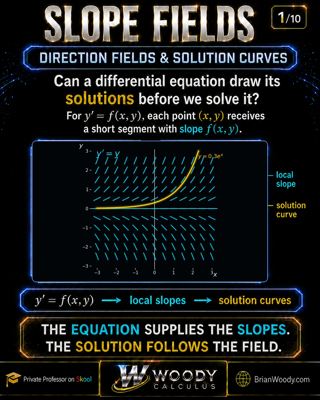
The differential equation is a local instruction
Consider a first-order differential equation written in explicit form:
y^{\prime}=f(x,y).
\]
The right-hand side does not immediately give the height of a solution. It gives the instantaneous slope a solution must have if it passes through the point \((x,y)\). At a particular point \((x_0,y_0)\), the required slope is
m=f(x_0,y_0).
\]
The slope field records that number with a short line segment centered at \((x_0,y_0)\). Repeating the process across a grid turns the algebraic rule \(f(x,y)\) into a geometric landscape.
For example, in
y^{\prime}=y,
\]
every point on the horizontal line \(y=2\) receives slope \(2\), every point on \(y=-1\) receives slope \(-1\), and every point on \(y=0\) receives slope \(0\). The equation depends on \(y\) but not on \(x\), so the field repeats along horizontal rows.
The exact solution family is
y=Ce^x.
\]
Differentiating verifies the tangency rule:
y^{\prime}=Ce^x=y.
\]
Slide 1 highlights the specific member \(y=0.3e^x\). At every point on that curve, the curve’s derivative equals its current height, which is exactly the slope encoded by the surrounding field.
How to read signs and steepness
| Value of \(f(x,y)\) | Segment appearance | What a solution does locally |
|---|---|---|
| \(f(x,y)>0\) | Rises from left to right | Increases as \(x\) increases |
| \(f(x,y)<0\) | Falls from left to right | Decreases as \(x\) increases |
| \(f(x,y)=0\) | Horizontal | Has a horizontal tangent there |
| \(|f(x,y)|\) small | Nearly horizontal | Changes slowly |
| \(|f(x,y)|\) large | Steep | Changes rapidly |
The segments should normally have equal geometric length. Their angles encode slope. If segment lengths vary with \(|f|\), a steep region can dominate the picture and make comparisons harder.
A slope field is not a graph of \(f\)
This distinction is essential. The surface \(z=f(x,y)\) would graph the numerical value of the right-hand side in three dimensions. A slope field stays in the \(xy\)-plane and converts each value \(f(x,y)\) into a local orientation.
It is often useful to imagine the two-dimensional vector
\langle 1,f(x,y)\rangle.
\]
Its slope is \(f(x,y)/1=f(x,y)\). The conventional slope-field dash is the unoriented line determined by that vector; when we follow a solution as \(x\) increases, we move from left to right.
What the field can reveal without an exact formula
A well-drawn direction field can answer qualitative questions before we solve anything:
- Where are solutions increasing or decreasing?
- Where can a solution have a local maximum or minimum?
- Which constant solutions are equilibria?
- Do nearby solutions approach or move away from an equilibrium?
- Does a solution appear bounded?
- Is there a curve that solutions approach asymptotically?
- Does the field become undefined along a singular line?
- How sensitive is the behavior to the initial condition?
This is why slope fields matter even when an exact solution exists. They expose the geometry that the formula may hide.
Part II — How to Construct a Slope Field by Hand
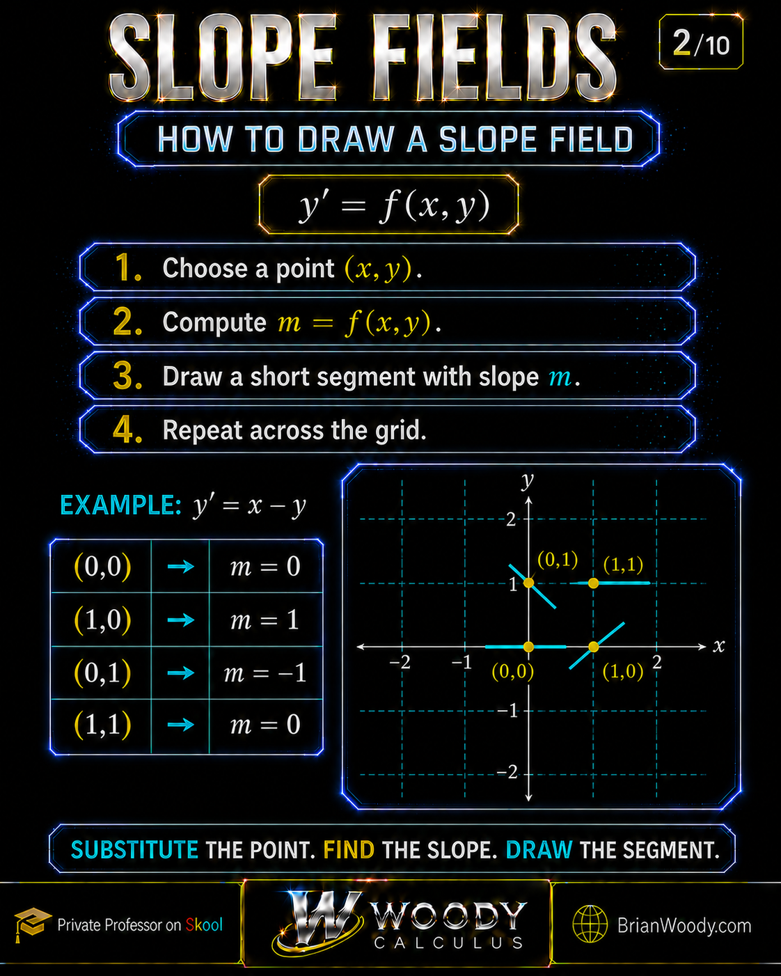
We will construct representative segments for
y^{\prime}=x-y.
\]
At every point, subtract the \(y\)-coordinate from the \(x\)-coordinate.
Four sample points
| Point \((x,y)\) | Compute \(x-y\) | Required slope | Segment |
|---|---|---|---|
| \((0,0)\) | \(0-0\) | \(0\) | Horizontal |
| \((1,0)\) | \(1-0\) | \(1\) | Rises at \(45^\circ\) on equal-scale axes |
| \((0,1)\) | \(0-1\) | \(-1\) | Falls at \(45^\circ\) on equal-scale axes |
| \((1,1)\) | \(1-1\) | \(0\) | Horizontal |
The computational loop is deliberately simple:
\text{choose point}
\longrightarrow
\text{evaluate }f(x,y)
\longrightarrow
\text{draw a short segment}
\longrightarrow
\text{repeat}.
\]
Converting a numerical slope into an angle
If a segment has slope \(m\), its angle \(\theta\) from the positive horizontal direction satisfies
\tan\theta=m,
\qquad
\theta=\arctan(m).
\]
You do not need a calculator for the common values used in a hand sketch:
| Slope | Visual angle |
|---|---|
| \(0\) | Horizontal |
| \(1\) | \(45^\circ\) upward |
| \(-1\) | \(45^\circ\) downward |
| \(2\) | Steeper than \(45^\circ\) upward |
| \(-2\) | Steeper than \(45^\circ\) downward |
| \(1/2\) | Shallow upward |
| \(-1/2\) | Shallow downward |
The exact visual angle depends on the graph’s axis scaling. A \(45^\circ\) segment represents slope \(1\) only when one unit in the \(x\)-direction occupies the same physical distance as one unit in the \(y\)-direction. This is one reason mathematically accurate slope-field graphics require controlled, uniform axes.
Start strategically, not randomly
For an exam sketch, do not compute every visible point immediately. Begin with structure:
- Find where \(f(x,y)=0\). These segments are horizontal.
- Find simple isoclines such as \(f(x,y)=1\) and \(f(x,y)=-1\).
- Evaluate points on the coordinate axes.
- Look for repeated rows, columns, diagonals, or symmetry.
- Fill only enough intermediate segments to make the pattern unmistakable.
For \(y^{\prime}=x-y\), the zero-slope equation is
x-y=0
\quad\Longleftrightarrow\quad
y=x.
\]
Thus every point on the diagonal \(y=x\) receives a horizontal dash. Above that diagonal, \(y>x\), so (x-y<0) and the segments fall. Below it, (x>y), so \(x-y>0\) and the segments rise.
That sign analysis already reveals the field’s main architecture.
Do not draw arrows of changing length
A slope field is not ordinarily a magnitude plot. The clean convention is to draw short segments of a common length and use only their orientation. Long arrows in steep regions can overlap neighboring segments, distort density, and make a finite slope look like explosive motion.
The quantity \(f(x,y)\) is a derivative, not a speed through the plane. We are graphing tangent directions to functions \(y(x)\), not particles whose two-dimensional velocity magnitude equals \(|f(x,y)|\).
Part III — Recognize the Pattern Before Calculating Everything
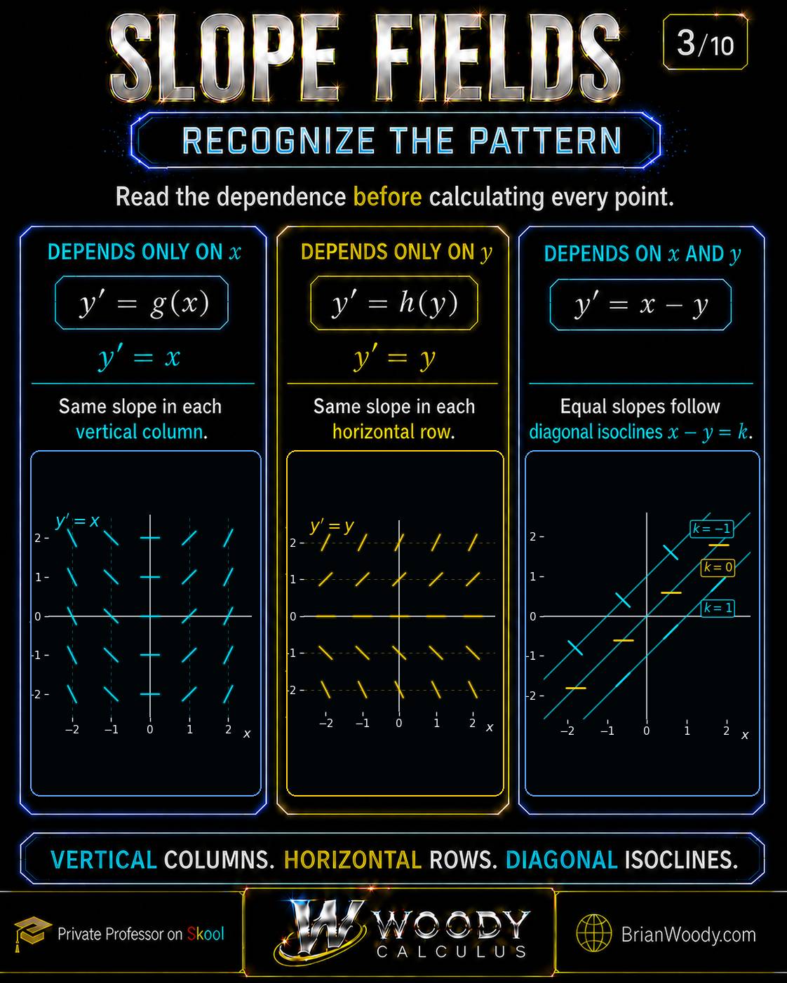
The dependence structure of \(f(x,y)\) predicts the repetition pattern in the field.
| Differential equation | What the slope depends on | Repetition pattern |
|---|---|---|
| \(y^{\prime}=g(x)\) | \(x\) only | Same slope in each vertical column |
| \(y^{\prime}=h(y)\) | \(y\) only | Same slope in each horizontal row |
| \(y^{\prime}=f(x,y)\) | Both variables | Often organized by isoclines |
| \(y^{\prime}=g(x)h(y)\) | Product of two factors | Sign regions from the signs of both factors |
Pattern 1: \(y^{\prime}=g(x)\) produces vertical columns
If
y^{\prime}=x,
\]
then every point with the same \(x\)-coordinate receives the same slope, regardless of height. Along \(x=-2\), the slope is \(-2\). Along \(x=0\), the slope is \(0\). Along \(x=2\), the slope is \(2\).
The exact solution family confirms the geometry:
y=\frac{x^2}{2}+C.
\]
Every member is a vertical translate of the same parabola, so every member has the same derivative \(y^{\prime}=x\) at a given \(x\).
Pattern 2: \(y^{\prime}=h(y)\) produces horizontal rows
If
y^{\prime}=y,
\]
then slope depends only on height. Every point on \(y=1\) has slope \(1\); every point on \(y=-2\) has slope \(-2\). This is the characteristic horizontal-band structure of an autonomous scalar equation.
The sign of \(h(y)\) can often be read as a one-dimensional phase line:
- \(h(y)>0\): solutions move upward as \(x\) increases.
- \(h(y)<0\): solutions move downward.
- \(h(y)=0\): the horizontal line may be an equilibrium solution.
Pattern 3: \(y^{\prime}=x-y\) produces diagonal isoclines
Fix the slope equal to a constant \(k\):
x-y=k.
\]
Solving for \(y\) gives
y=x-k.
\]
Each value of \(k\) produces a diagonal line, and every segment along that line has slope \(k\). The slope field is therefore organized into parallel diagonal bands.
Recognition can identify the equation from the picture
Suppose you are given a field and several candidate equations.
- Look for horizontal-row repetition. If present, favor an equation depending only on \(y\).
- Look for vertical-column repetition. If present, favor an equation depending only on \(x\).
- Locate the horizontal segments. Their coordinates must satisfy \(f(x,y)=0\).
- Check signs in test regions. A point above a zero isocline may have a different sign from one below it.
- Compare steepness. Distinguish slopes \(1\), \(2\), and \(1/2\); do not use sign alone.
- Check where the equation is undefined. A missing row, column, or curve may reveal a denominator or square-root restriction.
Example: distinguish three similar-looking equations
Compare
y^{\prime}=x,
\qquad
y^{\prime}=y,
\qquad
y^{\prime}=x-y.
\]
- The first repeats vertically and has horizontal segments on the \(y\)-axis.
- The second repeats horizontally and has horizontal segments on the \(x\)-axis.
- The third repeats along diagonal lines and has horizontal segments on \(y=x\).
One structural observation can replace dozens of point calculations.
Part IV — Isoclines, Zero-Slope Curves, and Equilibria
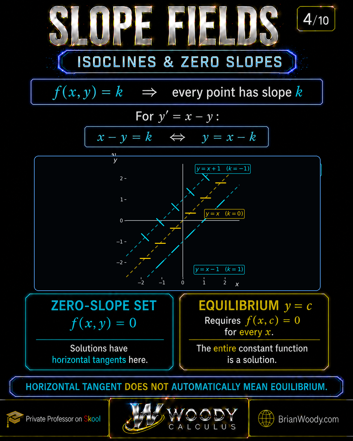
What is an isocline?
For
y^{\prime}=f(x,y),
\]
an isocline of slope \(k\) is a curve satisfying
f(x,y)=k.
\]
Every point on that curve receives a segment of slope \(k\). Isoclines organize a field by grouping points with identical derivative values.
For the running equation \(y^{\prime}=x-y\):
| Chosen slope \(k\) | Solve \(x-y=k\) | Isocline | Segment slope |
|---|---|---|---|
| \(-1\) | \(x-y=-1\) | \(y=x+1\) | \(-1\) |
| \(0\) | \(x-y=0\) | \(y=x\) | \(0\) |
| \(1\) | \(x-y=1\) | \(y=x-1\) | \(1\) |
These three lines explain most of the field. Additional values of \(k\) fill in parallel lines between and beyond them.
Zero isocline versus nullcline
In a scalar equation \(y^{\prime}=f(x,y)\), the set
f(x,y)=0
\]
is the zero-slope isocline. It is also commonly called a \(y\)-nullcline because the \(y\)-derivative vanishes there.
At any point where a genuine solution crosses this set, the solution has a horizontal tangent. But the set itself need not be a solution.
Why \(y=x\) is not a solution of \(y^{\prime}=x-y\)
Along the line \(y=x\), the differential equation requires
y^{\prime}=x-y=0.
\]
But the derivative of the proposed line \(y=x\) is
y^{\prime}=1.
\]
Because \(1\ne0\), the line \(y=x\) is not a solution. It merely identifies the points at which actual solutions have horizontal tangents.
This is one of the most important conceptual distinctions in the topic:
Horizontal tangent does not automatically mean equilibrium.
What is an equilibrium solution?
A constant function
y(x)=c
\]
has derivative \(y^{\prime}=0\). It is an equilibrium solution precisely when
f(x,c)=0
\]
for every \(x\) in the interval under consideration.
For an autonomous equation
y^{\prime}=g(y),
\]
every root \(g(c)=0\) produces the horizontal equilibrium \(y=c\). That is why equilibria appear naturally in horizontal rows for autonomous fields.
For the nonautonomous equation \(y^{\prime}=x-y\), there is no constant \(c\) satisfying \(x-c=0\) for every \(x\). Therefore it has no constant equilibrium solution, even though it has the zero-slope line \(y=x\).
Isoclines can also reveal turning points
Suppose a solution moves from a region where (f<0) into a region where (f>0). At the zero isocline, its slope is zero; the curve typically changes from decreasing to increasing and has a local minimum.
If it moves from \(f>0\) to \(f<0\), it typically has a local maximum.
The word “typically” matters because the curve’s direction of crossing and higher-order behavior must still be checked. In the complete example later, the solution crosses \(y=x\) at \((\ln2,\ln2)\), and direct differentiation confirms that the point is a strict minimum.
Part V — Solution Curves and Initial-Value Problems
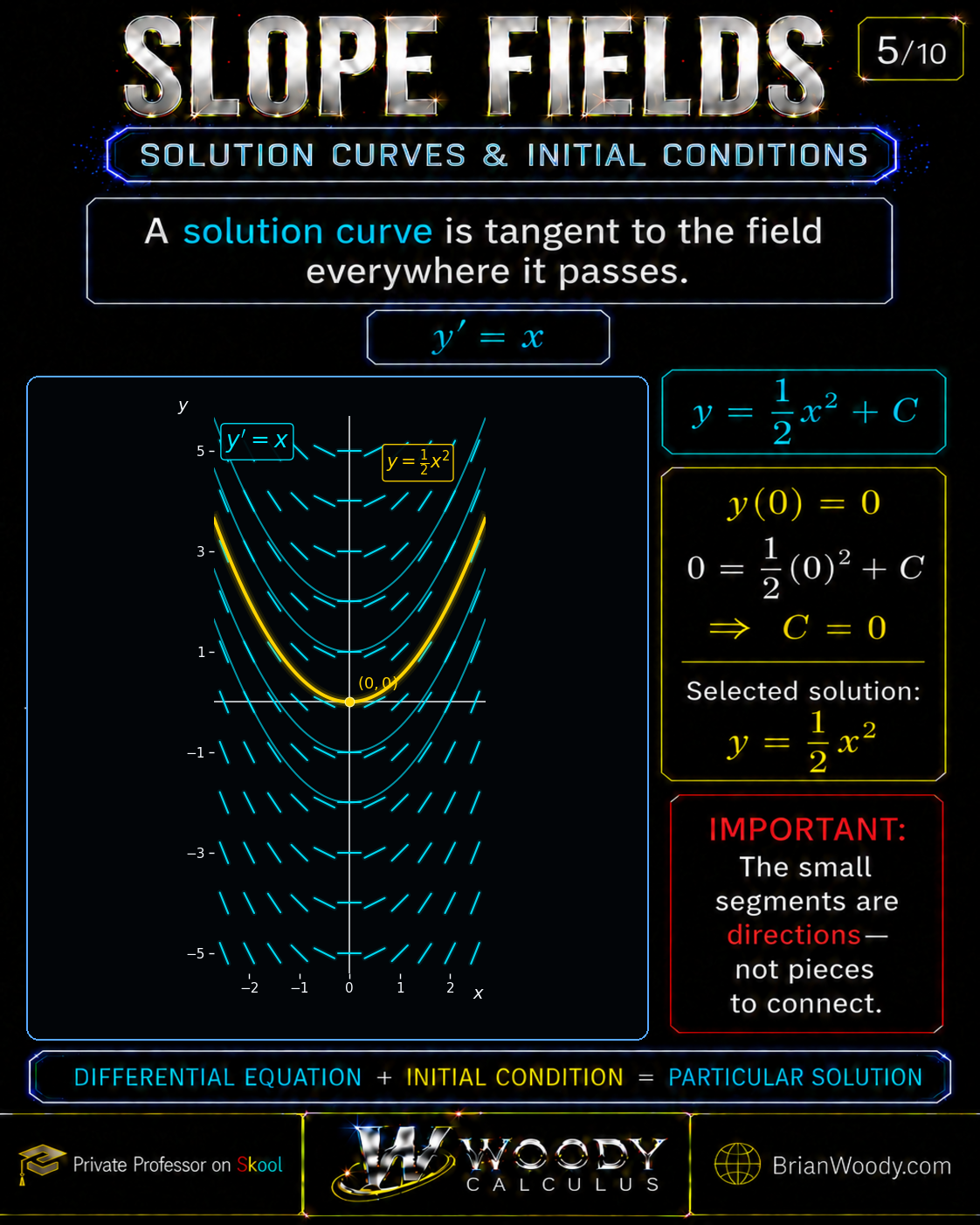
The field represents a family of solutions
Return to
y^{\prime}=x.
\]
Integrating gives
y=\frac{x^2}{2}+C.
\]
Different values of \(C\) produce vertical translates of the same parabola. Every curve is tangent to the same slope field because every curve has derivative \(x\).
The direction field therefore belongs to the differential equation, not to a particular value of \(C\).
An initial condition selects one curve
Add the condition
y(0)=0.
\]
Substitute into the general solution:
0=\frac{0^2}{2}+C,
\qquad
C=0.
\]
The selected solution is
\boxed{y=\frac{x^2}{2}.}
\]
Geometrically, the initial condition supplies a point. The field supplies the allowable tangent at that point and at every point the curve reaches.
The segments are directions, not pieces to connect
A common student error is to draw a polygon by joining the endpoints of neighboring dashes. That is not how a solution curve is constructed.
The dashes are centered at fixed sample points and show local directions. A solution curve should be smooth when the differential equation is smooth, and it should pass through the field, staying tangent to nearby segments. It does not need to touch the endpoints of the dashes.
Euler’s method does create a polygonal approximation, but even there the line segments begin at successive approximation points. They are not obtained by connecting the printed field marks.
Forward and backward sketching
Given \(y(x_0)=y_0\), sketch in both directions:
- To the right, follow the slopes as \(x\) increases.
- To the left, trace the same solution backward as \(x\) decreases.
At each step ask:
- Is the slope positive, negative, or zero?
- Is the curve becoming steeper or flatter?
- Is it approaching a zero isocline or equilibrium?
- Does the field indicate a turning point?
- Is there an undefined curve that the solution cannot cross within the classical problem?
Verification remains the final authority
A visually plausible curve is not automatically a solution. If a formula is available, differentiate it and check
y^{\prime}(x)=f(x,y(x)).
\]
For \(y=x^2/2+C\):
y^{\prime}=x,
\]
so every member satisfies the differential equation. For the IVP curve \(y=x^2/2\), we also verify \(y(0)=0\).
What a field cannot determine by itself
A finite grid is a sampled picture. It may hide behavior between grid points, beyond the viewing window, or near a singularity. It also does not prove global existence, uniqueness, boundedness, or convergence. Those claims require analysis.
Use the field to form a mathematically informed prediction. Then use algebra, calculus, and theorems to justify the prediction.
Part VI — Existence, Uniqueness, and Why Solutions Usually Do Not Cross
The standard local theorem
For the initial-value problem
y^{\prime}=f(x,y),
\qquad
y(x_0)=y_0,
\]
a standard sufficient condition is:
- \(f\) is continuous near \((x_0,y_0)\), and
- \(f\) is locally Lipschitz in \(y\) there.
Then a solution exists on some interval around \(x_0\) and is locally unique.
In many introductory courses, the easier-to-check hypothesis is that both \(f\) and \(f_y=\partial f/\partial y\) are continuous on a rectangle containing the initial point. Continuity of \(f_y\) implies the needed local Lipschitz control in \(y\).
Why uniqueness prevents two solution curves from crossing
Suppose two distinct solution curves passed through the same point \((x_*,y_*)\). Both would solve the same IVP
y^{\prime}=f(x,y),
\qquad
y(x_*)=y_*.
\]
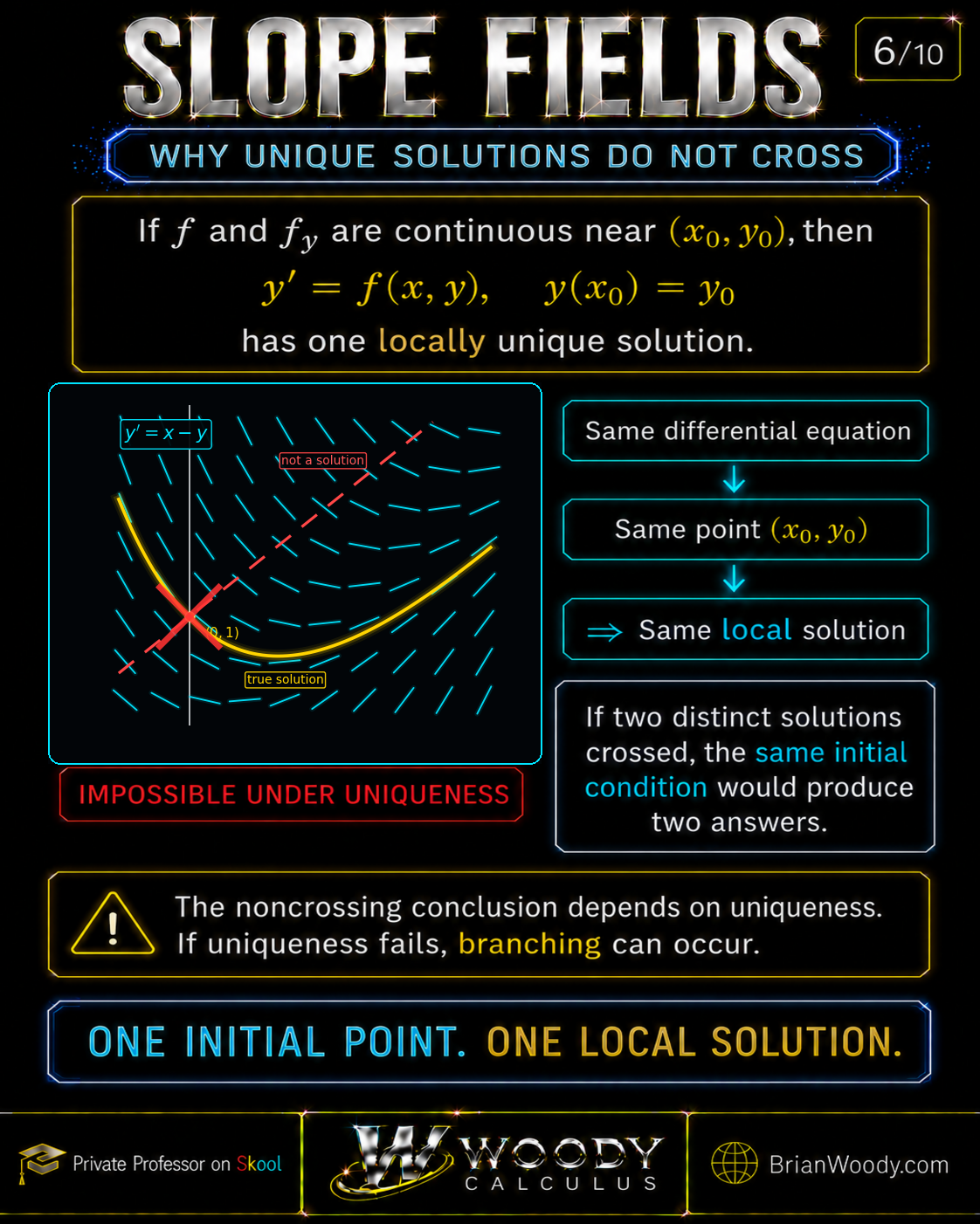
If the uniqueness hypotheses hold near that point, the IVP has only one local solution. The two curves must therefore coincide locally; they cannot cross and then separate as distinct solutions.
At the crossing point, the differential equation also assigns only one slope \(f(x_*,y_*)\). A proposed second curve with a different tangent fails immediately: it is not a solution.
Slide 6 uses the running example \(y^{\prime}=x-y\). The gold curve is
y=x-1+2e^{-x},
\]
and it passes through \((0,1)\). Its slope there is
y^{\prime}(0)=1-2=-1,
\]
which agrees with the field:
f(0,1)=0-1=-1.
\]
The red dashed candidate passes through the same point with the wrong tangent, so it fails the differential equation and is not a second solution.
Continuity alone does not guarantee uniqueness
Consider
y^{\prime}=3y^{2/3},
\qquad
y(0)=0.
\]
The right-hand side is continuous, so existence is not surprising. But uniqueness fails. Both
y=0
\]
and
y=x^3
\]
satisfy the equation and the initial condition. Indeed,
\frac{d}{dx}(x^3)=3x^2
\]
and
3(x^3)^{2/3}=3x^2.
\]
The derivative \(f_y=2y^{-1/3}\) is not continuous at \(y=0\), and the local Lipschitz condition fails there. This is exactly the kind of exception the theorem warns us about.
Local uniqueness is not global existence
Even a very smooth differential equation can have a solution that blows up in finite time. For example,
y^{\prime}=y^2,
\qquad
y(0)=1
\]
has the unique solution
y=\frac{1}{1-x},
\]
which becomes unbounded at \(x=1\). The theorem guarantees a unique solution near \(x=0\), not necessarily for every real \(x\).
The correct no-crossing statement
Do not memorize the unconditional sentence “solution curves never cross.” Use the precise statement:
In a region where the IVP is locally unique, two distinct solution curves cannot pass through the same point.
That version is mathematically accurate and remains valid when the course advances to singular equations and nonlinear examples.
Part VII — Complete Worked Example: \(y^{\prime}=x-y, y(0)=1\)
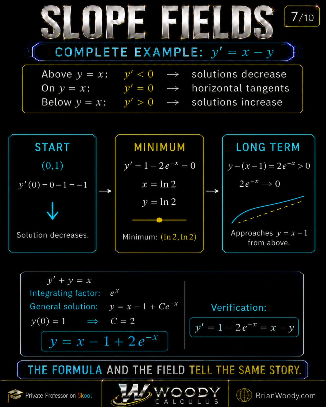
This example unifies the entire lesson: field pattern, isoclines, exact solution, initial condition, turning point, concavity, and asymptotic behavior.
Step 1: Put the equation in linear form
y^{\prime}=x-y
\]
becomes
y^{\prime}+y=x.
\]
Thus
P(x)=1,
\qquad
Q(x)=x.
\]
Step 2: Find the integrating factor
\mu(x)=e^{\int 1\,dx}=e^x.
\]
Multiply every term by \(e^x\):
e^xy^{\prime}+e^xy=xe^x.
\]
The left side is a product derivative:
\frac{d}{dx}(e^xy)=xe^x.
\]
Step 3: Integrate
Integration by parts gives
\int xe^x\,dx=e^x(x-1)+C.
\]
Therefore
e^xy=e^x(x-1)+C.
\]
Divide by \(e^x\):
y=x-1+Ce^{-x}.
\]
Step 4: Apply the initial condition
Use \(y(0)=1\):
1=0-1+C,
\]
so
C=2.
\]
The particular solution is
\boxed{y=x-1+2e^{-x}.}
\]
Step 5: Verify the differential equation
Differentiate:
y^{\prime}=1-2e^{-x}.
\]
Compute the right-hand side:
x-y
=x-\left(x-1+2e^{-x}\right)
=1-2e^{-x}.
\]
Hence
y^{\prime}=x-y.
\]
The initial condition also checks:
y(0)=-1+2=1.
\]
Step 6: Locate the horizontal tangent
Set \(y^{\prime}=0\):
1-2e^{-x}=0.
\]
Then
e^{-x}=\frac12,
\qquad
x=\ln2.
\]
Evaluate the solution:
y(\ln2)
=\ln2-1+2e^{-\ln2}
=\ln2-1+1
=\ln2.
\]
The horizontal tangent occurs at
\boxed{(\ln2,\ln2).}
\]
This point lies on the zero isocline \(y=x\), exactly as the slope field predicts.
Step 7: Confirm that the turning point is a minimum
Differentiate again:
y^{\prime\prime}=2e^{-x}>0
\]
for every real \(x\). The solution is concave up everywhere, so the horizontal tangent is a strict minimum.
Step 8: Read the long-term behavior
As \(x\to\infty\),
2e^{-x}\to0.
\]
Therefore
y-(x-1)=2e^{-x}\to0^+.
\]
The solution approaches the slant asymptote
\boxed{y=x-1}
\]
from above.
Notice that \(y=x-1\) is the \(k=1\) isocline. It is also a particular solution of the differential equation because its derivative is \(1\) and \(x-(x-1)=1\). This differs sharply from the zero isocline \(y=x\), which is not a solution.
The full geometry in one table
| Feature | Exact calculation | Field interpretation |
|---|---|---|
| Initial point | \(y(0)=1\) | Select the curve through \((0,1)\) |
| Initial slope | \(f(0,1)=-1\) | Curve initially decreases |
| Zero isocline | \(y=x\) | Horizontal dashes |
| Turning point | \((\ln2,\ln2)\) | Curve crosses \(y=x\) with slope \(0\) |
| Concavity | \(y^{\prime\prime}=2e^{-x}>0\) | Turning point is a minimum |
| Asymptote | \(y=x-1\) | Curve approaches the \(k=1\) isocline from above |
This is the payoff of slope fields: the exact analysis and the picture reinforce each other at every stage.
Part VIII — Autonomous Equations, Equilibria, and Stability
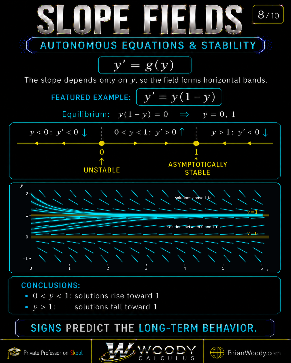
An autonomous scalar differential equation has the form
y^{\prime}=g(y).
\]
Because the right-hand side does not depend explicitly on \(x\), the field repeats along horizontal rows. This makes equilibrium and stability analysis especially efficient.
Logistic example
Consider
y^{\prime}=y(1-y).
\]
Equilibria occur when
y(1-y)=0,
\]
so
\boxed{y=0}
\qquad\text{and}\qquad
\boxed{y=1}.
\]
Build the sign chart
| Interval | Test value | Sign of \(y(1-y)\) | Motion as \(x\) increases |
|---|---|---|---|
| \(y<0\) | \(-1\) | Negative | Downward |
| \(0<y<1\) | \(1/2\) | Positive | Upward |
| \(y>1\) | \(2\) | Negative | Downward |
Near \(y=0\), solutions on both sides move away from the equilibrium: below \(0\) they move downward, and above \(0\) they move upward. Thus \(y=0\) is unstable.
Near \(y=1\), solutions below move upward and solutions above move downward. Both sides move toward the equilibrium, so \(y=1\) is asymptotically stable.
Phase-line notation
The same information can be compressed into a vertical phase line:
(-\infty,0):\downarrow,
\qquad
0,
\qquad
(0,1):\uparrow,
\qquad
1,
\qquad
(1,\infty):\downarrow.
\]
The phase line is not the same as a two-dimensional phase portrait. It records one state variable \(y\) and its direction of change. A phase portrait studies a system such as
x^{\prime}=F(x,y),
\qquad
y^{\prime}=G(x,y)
\]
in the phase plane. For that next step, use the Woody Calculus lesson on phase portraits and stability.
General logistic equation
The standard logistic model is
P^{\prime}=rP\left(1-\frac{P}{K}\right),
\qquad
r>0, K>0.
\]
The equilibria are \(P=0\) and \(P=K\). For physically meaningful initial populations \(P_0>0\):
- if \(0<P_0<K\), the population increases toward \(K\);
- if \(P_0>K\), the population decreases toward \(K\);
- if \(P_0=K\), the population remains at carrying capacity.
The field reveals this behavior without requiring the explicit logistic formula.
Stability is a local directional statement
To classify an equilibrium \(y=c\), inspect the signs immediately above and below it:
- arrows toward \(c\) from both sides: asymptotically stable;
- arrows away from \(c\) from both sides: unstable;
- toward on one side and away on the other: semistable.
Do not decide stability from the flat equilibrium line alone. Stability depends on what nearby solutions do.
Equilibrium barriers and uniqueness
When uniqueness holds, a non-equilibrium solution cannot cross an equilibrium solution. If it reached \(y=c\) at some finite \(x_*\), both the nonconstant curve and the equilibrium \(y=c\) would solve the IVP through \((x_*,c)\), contradicting uniqueness.
This theorem explains why many slope fields show neighboring curves approaching an equilibrium asymptotically without crossing it.
Part IX — Euler’s Method as a Walk Through the Slope Field
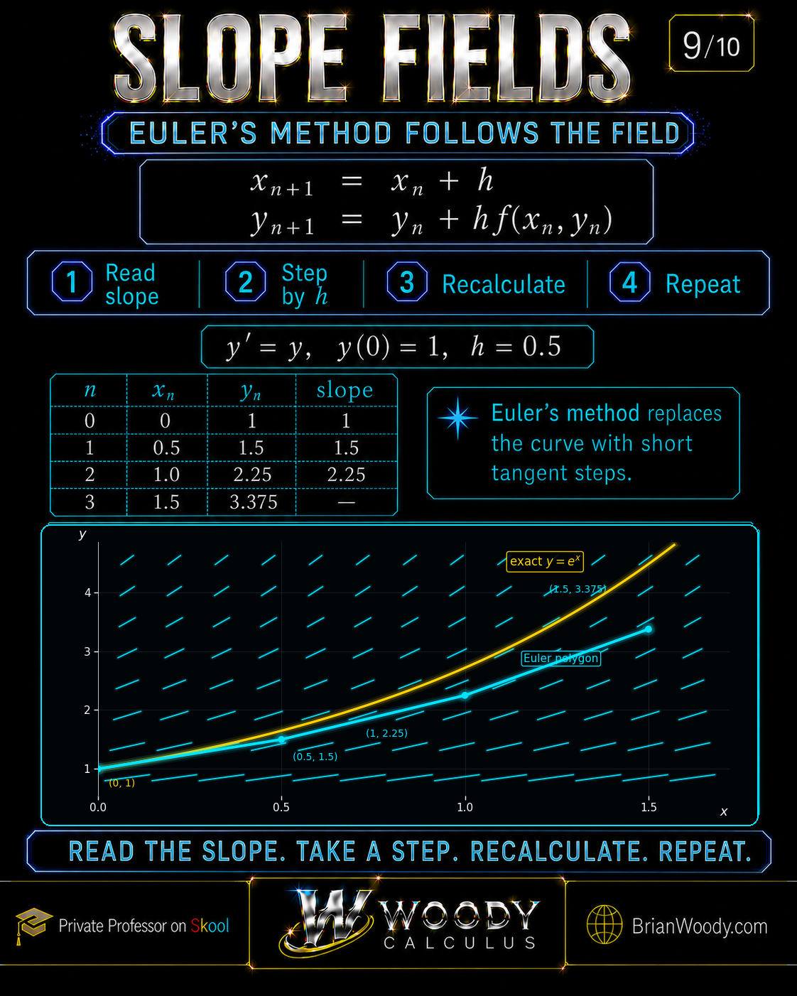
Euler’s method turns local slope information into a numerical approximation.
For
y^{\prime}=f(x,y),
\qquad
y(x_0)=y_0,
\]
choose a step size \(h\) and iterate
\boxed{
x_{n+1}=x_n+h,
\qquad
y_{n+1}=y_n+h f(x_n,y_n).
}
\]
The method freezes the slope at the current point, follows that tangent for one horizontal step, evaluates the new slope, and repeats.
Worked Euler table for \(y^{\prime}=y\)
Use
y^{\prime}=y,
\qquad
y(0)=1,
\qquad
h=0.5.
\]
Because \(f(x,y)=y\), the update is
y_{n+1}=y_n+0.5y_n=1.5y_n.
\]
| \(n\) | \(x_n\) | \(y_n\) | Slope \(f(x_n,y_n)=y_n\) | Update |
|---|---|---|---|---|
| 0 | \(0\) | \(1\) | \(1\) | \(y_1=1+0.5(1)=1.5\) |
| 1 | \(0.5\) | \(1.5\) | \(1.5\) | \(y_2=1.5+0.5(1.5)=2.25\) |
| 2 | \(1.0\) | \(2.25\) | \(2.25\) | \(y_3=2.25+0.5(2.25)=3.375\) |
Thus
\boxed{y(1.5)\approx3.375.}
\]
The exact solution is
y=e^x,
\]
so
e^{1.5}\approx4.481689.
\]
The absolute error is approximately
4.481689-3.375=1.106689,
\]
and the relative error is approximately \(24.69\%\).
Why Euler undershoots this exponential
The exact solution \(e^x\) is concave up because
y^{\prime\prime}=e^x>0.
\]
For a concave-up curve, each tangent line lies below the graph near the point of tangency. Forward Euler follows those left-endpoint tangents, so the polygonal approximation remains below the exact curve in this example.
This is not a universal rule that Euler always underestimates. The direction of the error depends on the solution’s curvature, the step direction, and the problem.
Step size and accuracy
For the same IVP at \(x=1.5\):
| Step size \(h\) | Number of steps | Euler value | Absolute error | Relative error |
|---|---|---|---|---|
| \(0.5\) | 3 | \(3.375000\) | \(1.106689\) | \(24.69\%\) |
| \(0.25\) | 6 | \(3.814697\) | \(0.666992\) | \(14.88\%\) |
| \(0.1\) | 15 | \(4.177248\) | \(0.304441\) | \(6.79\%\) |
Smaller \(h\) usually improves the approximation for a smooth, well-behaved IVP because the slope is refreshed more frequently. Under standard smoothness assumptions, forward Euler has local truncation error of order \(O(h^2)\) per step and accumulated global error of order \(O(h)\) over a fixed interval.
Slope field versus Euler polygon
| Slope field | Euler approximation |
|---|---|
| Displays slopes at many fixed grid points | Uses slopes only at the computed Euler points |
| Describes an entire family of possible solutions | Approximates one IVP solution |
| Gives qualitative geometry | Gives numerical values |
| Uses short centered dashes | Uses connected tangent-line steps |
| Does not require a step size | Requires a chosen \(h\) |
For a complete numerical treatment, continue to Euler’s Method Explained.
Euler’s method is the computational version of the picture
The field says, “At this point, this is the allowed slope.” Euler’s method responds, “Follow that slope for a short distance, then ask again.” More advanced Runge–Kutta methods improve the decision by sampling multiple slopes within each step, but the central geometric idea remains local slope information guiding global motion.
Part X — Reading Unknown Fields, Common Mistakes, and Mastery
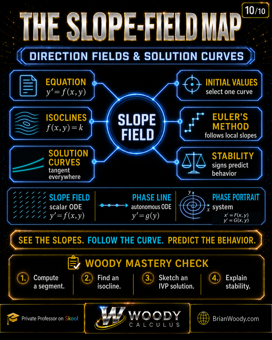
Slope field, phase line, and phase portrait
These related pictures answer different questions.
| Tool | Typical equation | Plane or axis | Main purpose |
|---|---|---|---|
| Slope field | \(y^{\prime}=f(x,y)\) | \(x\)–\(y\) plane | Show tangents to graphs \(y(x)\) |
| Phase line | \(y^{\prime}=g(y)\) | One state axis | Classify scalar equilibria and stability |
| Phase portrait | \(x^{\prime}=F(x,y),\ y^{\prime}=G(x,y)\) | State-space \(x\)–\(y\) plane | Show trajectories of a two-dimensional system |
In a slope field, \(x\) is usually the independent variable and \(y\) is dependent. In a phase portrait, both coordinates are dependent variables evolving with time. The pictures may look related, but their axes mean different things.
How to analyze an unfamiliar slope field
Use this order:
- Find horizontal segments. They reveal \(f(x,y)=0\).
- Mark positive and negative regions. Decide where solutions rise or fall.
- Compare steepness. Track how \(|f|\) changes.
- Look for repetition. Rows suggest \(y\)-dependence; columns suggest \(x\)-dependence; diagonals suggest isoclines.
- Locate equilibria. A full horizontal row of zero slopes is a candidate, but verify that the constant line satisfies the equation for all \(x\).
- Look for singular sets. Missing or nearly vertical marks can signal an undefined right-hand side.
- Use the initial condition. Select the correct trajectory.
- Sketch tangentially. Do not connect field dashes.
- State long-term behavior carefully. Distinguish visual evidence from theorem-backed conclusions.
Can a slope field reveal concavity?
Yes, but the reasoning is subtler than reading the sign of \(y^{\prime}\). Along a solution \(y(x)\), differentiate the equation:
y^{\prime\prime}
=\frac{d}{dx}f(x,y(x))
=f_x(x,y)+f_y(x,y)y^{\prime}.
\]
Since \(y^{\prime}=f(x,y)\),
\boxed{y^{\prime\prime}=f_x+f_yf.}
\]
Geometrically, a solution is concave up where its encountered slopes increase as it moves right, and concave down where they decrease. But remember that the curve changes both \(x\) and \(y\), so scanning only a fixed row or column may be misleading.
Singularities and undefined slopes
Suppose
y^{\prime}=\frac{1}{x-y}.
\]
The right-hand side is undefined on \(y=x\). A correct direction field should not draw ordinary finite-slope segments there. Near that line, slopes become very large in magnitude.
An undefined set is not the same as a zero isocline:
- \(f=0\) means a horizontal tangent is required.
- \(f\) undefined means the explicit ODE does not assign a classical finite slope there.
Always inspect the domain before interpreting the picture.
Common mistakes
- Plotting \(f(x,y)\) as a height instead of a slope. The field belongs in the \(xy\)-plane.
- Using sign but ignoring magnitude. Slopes \(1/2\), \(1\), and (3) are all positive but geometrically different.
- Changing segment length with slope. Use equal-length dashes and change their angle.
- Connecting dash endpoints. A solution curve follows directions; it does not connect printed marks.
- Calling every zero isocline an equilibrium. Verify the constant function separately.
- Letting a proposed solution cut across the dashes. Tangency must hold everywhere.
- Claiming solutions never cross without checking uniqueness. State the theorem’s hypotheses.
- Ignoring where \(f\) is undefined. Singular sets can divide the domain and limit solutions.
- Forgetting the initial condition. The equation gives a family; the IVP selects one curve.
- Treating an Euler polygon as exact. Euler values are approximations unless independently proved otherwise.
- Confusing a scalar slope field with a system phase portrait. Read the axes and variables.
- Trusting a decorative plot without checking it. A mathematically valid field must match the printed equation point by point.
Woody Mastery Check
Without looking back, answer these aloud:
- What does the segment at \((x_0,y_0)\) represent?
- Why does \(y^{\prime}=g(x)\) repeat in vertical columns?
- Why does \(y^{\prime}=h(y)\) repeat in horizontal rows?
- What equation defines an isocline of slope \(k\)?
- Why is the zero isocline \(y=x\) not a solution of \(y^{\prime}=x-y\)?
- What additional condition turns a horizontal line into an equilibrium solution?
- Under what hypotheses can two solution curves not cross?
- Why does Euler’s method use the slope at the current point?
- Why does forward Euler undershoot \(e^x\) in the worked example?
- What is the difference between a slope field and a phase portrait?
Then redraw the core map from memory:
\boxed{
\text{equation}
\longrightarrow
\text{local slopes}
\longrightarrow
\text{isoclines and signs}
\longrightarrow
\text{solution curves}
\longrightarrow
\text{stability and approximation}.
}
\]
How to practice this lesson
Use the Woody Calculus repetition system:
- Rewrite the seven-step slope-field algorithm three to five times.
- Say each step aloud while drawing one field by hand.
- Practice matching equations to fields without calculating every point.
- For every zero-slope set, say whether it is merely an isocline or also an equilibrium.
- Sketch several IVP curves and check tangency.
- Solve one example exactly and compare the formula with the field.
- Run Euler’s method and explain the error geometrically.
The objective is automatic recognition: see the equation, anticipate the pattern, and explain the behavior before the algebra becomes complicated.
Where to go next
- Learn how to choose an analytic method with Separable vs. Linear Differential Equations.
- Develop the numerical workflow in Euler’s Method Explained.
- Move from scalar fields to systems with Phase Portraits and Stability.
- Explore the full Differential Equations Tutor and ODE Help pathway.
- Browse the complete Woody Calculus Math Library.
Slope Fields FAQ
What is a slope field in differential equations?
A slope field is a grid of short line segments for a first-order ODE \(y^{\prime}=f(x,y)\). The segment centered at \((x,y)\) has slope \(f(x,y)\), so solution curves must remain tangent to the displayed directions.
Are slope fields and direction fields the same thing?
Yes. In introductory differential equations, “slope field” and “direction field” usually refer to the same graphical representation of \(y^{\prime}=f(x,y)\).
How do you draw a slope field by hand?
Write the ODE as \(y^{\prime}=f(x,y)\), choose grid points, evaluate \(f\) at representative points, draw equal-length segments with those slopes, and use isoclines or repetition patterns to fill the grid efficiently.
What does each line segment in a slope field mean?
The segment at \((x_0,y_0)\) represents the tangent slope \(f(x_0,y_0)\) that any solution passing through that point must have.
How do positive and negative slopes appear?
Positive slopes rise from left to right, negative slopes fall from left to right, and zero slopes are horizontal. Larger absolute slope means a steeper segment.
Why do some slope fields repeat in horizontal rows?
If \(y^{\prime}=h(y)\) depends only on \(y\), every point at the same height has the same derivative. Therefore each horizontal row has a common slope.
Why do some slope fields repeat in vertical columns?
If \(y^{\prime}=g(x)\) depends only on \(x\), every point with the same \(x\)-coordinate has the same derivative. Therefore each vertical column has a common slope.
What is an isocline?
An isocline of slope \(k\) is a curve satisfying \(f(x,y)=k\). Every field segment along that curve has slope \(k\).
What is a nullcline in a slope field?
For a scalar equation \(y^{\prime}=f(x,y)\), the \(y\)-nullcline is the set \(f(x,y)=0\). It is the zero-slope isocline where solution curves have horizontal tangents.
Is a zero-slope isocline always a solution?
No. For \(y^{\prime}=x-y\), the zero isocline is \(y=x\), but that line has derivative \(1\) while the ODE requires slope \(0\) along it. It marks horizontal tangencies of actual solutions rather than being a solution itself.
What is an equilibrium solution?
An equilibrium solution is a constant function \(y=c\) satisfying \(f(x,c)=0\) for every relevant \(x\). For an autonomous equation \(y^{\prime}=g(y)\), equilibria are the roots of \(g(c)=0\).
What does an initial condition do in a slope field?
An initial condition \(y(x_0)=y_0\) selects the solution curve passing through \((x_0,y_0)\). The slope field then guides that curve locally in both directions.
Should I connect the small segments?
No. The printed segments are local direction markers, not endpoints to connect. Sketch a smooth curve through the field that stays tangent to the nearby segments.
Can two solution curves cross?
They cannot cross as distinct solutions in a region where the initial-value problem is locally unique. Without a uniqueness hypothesis, different solutions can pass through the same point.
What conditions guarantee a unique local solution?
A standard condition is that \(f(x,y)\) is continuous and locally Lipschitz in \(y\) near the initial point. A common sufficient test is continuity of both \(f\) and \(f_y\) on a surrounding rectangle.
Is continuity of the right-hand side enough for uniqueness?
No. Continuity can support existence, but uniqueness may fail without Lipschitz control in \(y\). The IVP \(y^{\prime}=3y^{2/3}, y(0)=0\) has both \(y=0\) and \(y=x^3\) as solutions.
Can a slope field give an exact solution?
A slope field is primarily qualitative. It can suggest the shape and behavior of solutions, but an exact formula requires analytic work or an independent verification.
How do I identify increasing and decreasing solutions?
Solutions increase in regions where \(f(x,y)>0\) and decrease where (f\(x,y\)<0). They have horizontal tangents where (f(x,y)=0).
Can a slope field show concavity?
Yes. A solution is concave up where the slopes it encounters increase as it moves right and concave down where they decrease. Analytically, \(y^{\prime\prime}=f_x+f_yf\) along a solution.
What happens where the differential equation is undefined?
The field should omit ordinary segments where \(f(x,y)\) is undefined. Such singular sets can divide the domain and restrict how classical solutions continue.
How is Euler’s method related to a slope field?
Euler’s method starts at an initial point, evaluates the field’s slope there, follows that tangent for one step, and repeats from the new approximation point.
Why does Euler’s method underestimate e^x in the example?
The exact solution \(e^x\) is concave up, so each forward tangent segment lies below the curve. This produces an underestimate for the displayed positive step size.
What is the difference between a slope field and a phase portrait?
A slope field for \(y^{\prime}=f(x,y)\) shows tangent directions to graphs \(y(x)\), with \(x\) as the independent variable. A phase portrait shows trajectories of a system in state space, where both plotted coordinates evolve with time.
Can software generate slope fields?
Yes. Graphing calculators, computer algebra systems, and numerical libraries can generate direction fields. The graph is trustworthy only when the equation, domain, axis scaling, and slope normalization are entered correctly.
What is the best way to practice slope fields?
Practice the complete loop: evaluate representative slopes, identify isoclines, mark sign regions, sketch an IVP curve, explain equilibrium behavior, and compare the picture with an exact or Euler solution. Rewrite the process and say each step aloud until it becomes automatic.
Master Slope Fields with Woody Calculus
Slope fields are where differential equations become visible. The equation gives local derivative data; isoclines organize that data; initial conditions select curves; uniqueness controls whether those curves can intersect; autonomous fields expose stability; and Euler’s method turns the same local information into numbers.
The complete method is:
\boxed{
\text{write }y^{\prime}=f(x,y)
\longrightarrow
\text{evaluate slopes}
\longrightarrow
\text{recognize patterns}
\longrightarrow
\text{sketch tangentially}
\longrightarrow
\text{verify behavior}.
}
\]
For structured help with first-order equations, slope fields, Euler’s method, Laplace transforms, systems, phase portraits, eigenvalues, and exam preparation, begin in the Woody Calculus Mastery Lab.
References
- OpenStax, Calculus Volume 2, Section 4.2, “Direction Fields and Numerical Methods.” https://openstax.org/books/calculus-volume-2/pages/4-2-direction-fields-and-numerical-methods
- Paul Dawkins, Lamar University, Paul’s Online Math Notes, “Direction Fields.” https://tutorial.math.lamar.edu/classes/de/directionfields.aspx
- Jiří Lebl, Differential Equations for Engineers, “Slope Fields” and Picard’s theorem, Mathematics LibreTexts. https://math.libretexts.org/Bookshelves/Differential_Equations/Differential_Equations_for_Engineers_%28Lebl%29/1%3A_First_order_ODEs/1.2%3A_Slope_fields
- Woody Calculus, “Euler’s Method Explained: Formula, Steps, Accuracy, and a Worked Example.” https://www.brianwoody.com/eulers-method-differential-equations-formula-example/
- Woody Calculus, “Phase Portraits Explained: Predict Stability from Eigenvalues.” https://www.brianwoody.com/phase-portraits-differential-equations-eigenvalues-stability/
- Woody Calculus, “Separable vs. Linear Differential Equations: How to Choose the Right Method.” https://www.brianwoody.com/separable-vs-linear-differential-equations-how-to-choose/