Number Theory • Abstract Algebra • Arithmetic Geometry • Visual Lesson
What Is Fermat’s Last Theorem?
Fermat’s Last Theorem states that no positive integers \(a,b,c\) satisfy \(a^n+b^n=c^n\) for any integer exponent \(n>2\). Andrew Wiles proved the theorem by establishing the modularity of semistable elliptic curves over \(\mathbb Q\). A hypothetical Fermat counterexample would produce a semistable Frey curve that Ribet’s theorem forces to be non-modular, while Wiles’s theorem forces it to be modular. The contradiction eliminates every possible counterexample.
The proof changes the object: equation → Frey curve → Galois representation → impossible modularity contradiction.
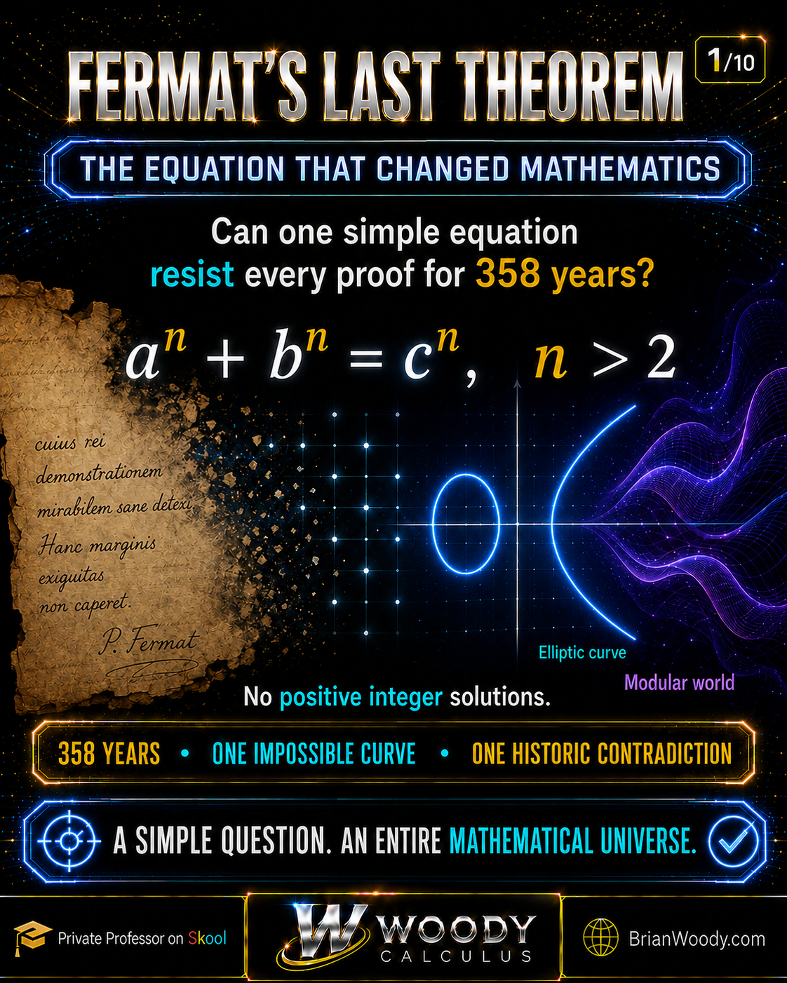
The Proof Architecture in Five Steps
This is the logical spine of the modern proof. The rest of the lesson builds the mathematics needed to justify every arrow.
- Assume a counterexample exists. Suppose positive integers a, b, and c satisfy a^p + b^p = c^p for an odd prime exponent p after the standard exponent reduction.
- Build the Frey curve. Attach the semistable elliptic curve E: y^2 = x(x – a^p)(x + b^p), whose arithmetic remembers the hypothetical solution.
- Apply Ribet’s level-lowering theorem. If the Frey curve were modular, its mod-p Galois representation would arise from a weight-two cusp form of level 2, but that space is zero; therefore the Frey curve cannot be modular.
- Apply Wiles–Taylor semistable modularity. Wiles’s modularity-lifting argument, completed with Taylor, proves that every semistable elliptic curve over the rational numbers is modular; therefore the Frey curve must be modular.
- Conclude by contradiction. The same Frey curve cannot be both modular and non-modular, so the assumed Fermat counterexample cannot exist.
What This Lesson Proves—and What It Does Not Claim
This lesson gives the complete logical architecture of Fermat’s Last Theorem and develops the central machinery with explicit proofs, derivations, and verified examples. It does not reproduce every technical local lemma in the original Wiles and Taylor–Wiles papers; those papers fill hundreds of pages and presuppose advanced arithmetic geometry.
Part I — The Problem Anyone Can Understand
There are equations that look difficult because they are covered in unfamiliar symbols. Fermat’s Last Theorem is the opposite. A middle-school student can understand the question, yet the proof ultimately required some of the deepest mathematics of the twentieth century.
Start with a familiar fact:
3^2+4^2=5^2.
\]
The three whole numbers \(3,4,5\) form the side lengths of a right triangle. They are one example among infinitely many integer solutions to
a^2+b^2=c^2.
\]
Now change one small thing. Replace the exponent \(2\) by \(3\), \(4\), \(5\), or any larger integer:
a^n+b^n=c^n.
\]
Can three positive whole numbers still make the equation work?
Fermat’s Last Theorem says no. Not once. Not for cubes, fourth powers, hundredth powers, or any integer exponent greater than \(2\).
That single claim resisted proof for centuries. It inspired ingenious partial results, created new branches of Number Theory, and eventually led mathematicians through algebraic number fields, ideals, elliptic curves, modular forms, and Galois representations. Andrew Wiles finally completed the essential breakthrough in the 1990s, not by attacking the original equation head-on, but by proving that a hypothetical solution would create a mathematical object that would have to be both modular and non-modular at the same time.
That contradiction is the destination of this lesson.
The journey begins here, with the equation itself.
Woody’s perspective. Woody studied the proof of Fermat’s Last Theorem in a year-long, two-semester course at the University of Wisconsin–Madison. This lesson is designed to preserve the excitement of that journey while building every bridge a motivated reader needs—from the elementary equation to the modern proof architecture.
What Is Fermat’s Last Theorem?
Here is the formal statement.
Fermat’s Last Theorem. If \(n\) is an integer greater than \(2\), then the equation \[
a^n+b^n=c^n
\] has no solution in positive integers \(a,b,c\).
Every phrase matters.
- Integer exponent: The exponent is one of \(3,4,5,\ldots\), not an arbitrary real number.
- Positive integers: The variables must be positive whole numbers. If zero were allowed, expressions such as \(a^n+0^n=a^n\) would create trivial solutions unrelated to the theorem.
- No solution: The theorem rules out every possible positive-integer triple, not merely the triples that have been checked so far.
- Greater than \(2\): The exponent \(2\) is deliberately excluded because it has infinitely many positive-integer solutions.
The theorem is a Diophantine statement: it asks for integer solutions to a polynomial equation. Closely related questions may ask for rational points, but Fermat’s Last Theorem concerns positive integers. Over the real numbers there is no mystery. Given positive real numbers \(a\) and \(b\), we can simply define
c=\left(a^n+b^n\right)^{1/n},
\]
and obtain a real solution. The extraordinary rigidity appears only when \(a,b,c\) are required to be integers.
The result is also easy to misread. It does not say that equations containing high powers never have integer solutions. For example,
2^3+2^3=2^4
\]
is true, but the three exponents are not all the same. Fermat’s equation requires the common exponent \(n\) on all three terms.
A theorem with an unusually long life
Fermat recorded his famous claim in the margin of a copy of Diophantus’s Arithmetica, conventionally dated around 1637. The note was published posthumously by his son Samuel in 1670. Fermat wrote that he had discovered a “truly marvelous” proof but that the margin was too narrow to contain it.
No general proof by Fermat survives.
For more than three centuries, the claim was known as Fermat’s Last Theorem even though it remained unproved. Wiles announced a proof in 1993; a gap was then discovered, and Wiles and Richard Taylor repaired the argument. The completed papers appeared in 1995—about 358 years after the date traditionally attached to Fermat’s note.
The phrase “Wiles proved Fermat’s Last Theorem” is correct, but it compresses a vast collaborative history. Fermat, Euler, Sophie Germain, Dirichlet, Legendre, Lamé, Kummer, Frey, Serre, Ribet, Taniyama, Shimura, Weil, Mazur, Taylor, and many others created the ideas that made the final argument possible. One of the central themes of this lesson will be that great proofs often arrive only after mathematics has developed the language in which the proof can exist.
Why the Exponent \(2\) Is Completely Different
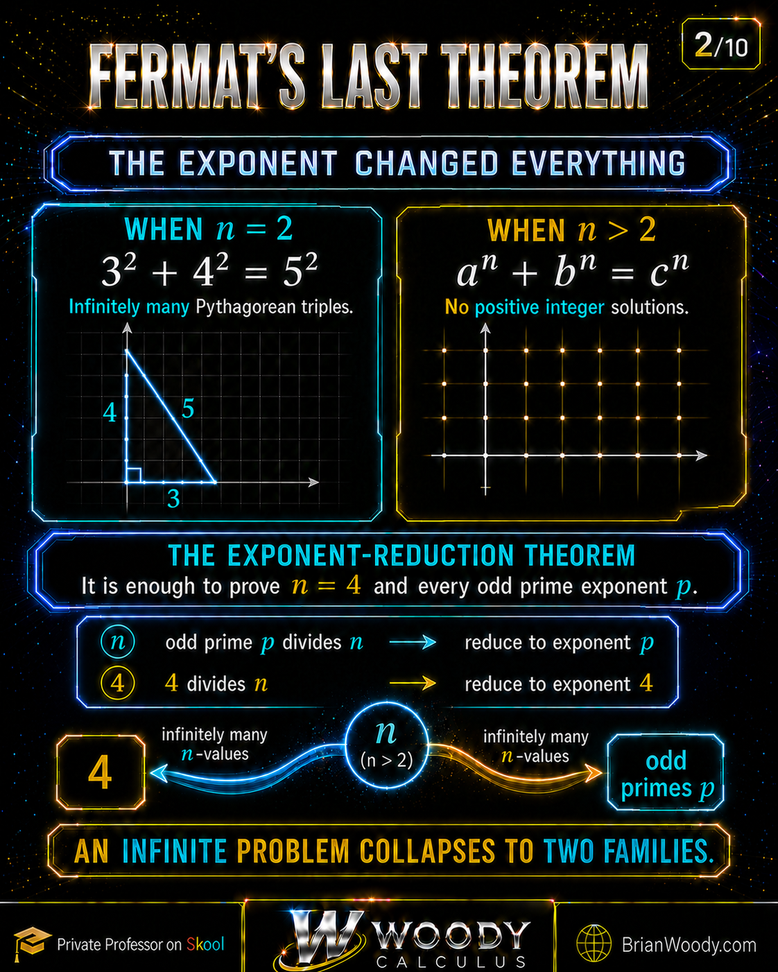
Fermat’s theorem begins at \(n=3\) because \(n=2\) belongs to a different mathematical world.
The equation
a^2+b^2=c^2
\]
is the Pythagorean equation. A positive-integer solution \((a,b,c)\) is called a Pythagorean triple. The most famous example is
3^2+4^2=5^2,
\]
because
9+16=25.
\]
But \((3,4,5)\) is not an isolated accident. There is a formula that generates infinitely many solutions.
Choose integers \(m>r>0\), and define
a=m^2-r^2,
\qquad
b=2mr,
\qquad
c=m^2+r^2.
\]
Then
\begin{aligned}
a^2+b^2
&=(m^2-r^2)^2+(2mr)^2\\
&=m^4-2m^2r^2+r^4+4m^2r^2\\
&=m^4+2m^2r^2+r^4\\
&=(m^2+r^2)^2\\
&=c^2.
\end{aligned}
\]
So the formulas produce a Pythagorean triple every time.
Worked example 1: generate \((3,4,5)\)
Let \(m=2\) and \(r=1\). Then
\begin{aligned}
a&=2^2-1^2=3,\\
b&=2(2)(1)=4,\\
c&=2^2+1^2=5.
\end{aligned}
\]
Therefore
3^2+4^2=5^2.
\]
Worked example 2: generate \((5,12,13)\)
Let \(m=3\) and \(r=2\). Then
\begin{aligned}
a&=3^2-2^2=5,\\
b&=2(3)(2)=12,\\
c&=3^2+2^2=13.
\end{aligned}
\]
Therefore
5^2+12^2=13^2,
\]
because
25+144=169.
\]
As \(m\) and \(r\) vary, these formulas generate infinitely many triples. If \(m\) and \(r\) are relatively prime and have opposite parity, the resulting triple is primitive, meaning \(a,b,c\) have no common factor greater than \(1\). Every primitive Pythagorean triple arises from this parametrization, up to exchanging the two shorter sides.
That is a remarkable contrast:
\boxed{a^2+b^2=c^2\text{ has infinitely many positive-integer solutions}}
\]
but
\boxed{a^n+b^n=c^n\text{ has none when }n>2.}
\]
The geometric intuition
At exponent \(2\), the equation describes right triangles and points on a conic. After dividing by \(c^2\), we obtain
\left(\frac{a}{c}\right)^2+
\left(\frac{b}{c}\right)^2=1.
\]
This is the unit circle. A line of rational slope through the rational point \((-1,0)\) meets the circle at one additional rational point, and that geometric construction leads to the Pythagorean parametrization.
For exponent \(n>2\), the corresponding Fermat curve
x^n+y^n=1
\]
has a fundamentally different arithmetic geometry. The shape may still look like a smooth curve over the real numbers, but its rational points become far more rigid. Much later in the lesson, this shift—from conics to higher-genus curves—will help explain why the innocent-looking change of exponent transforms the problem so completely.
For now, remember the central contrast:
Exponent \(2\) gives a construction. Exponents greater than \(2\) demand an impossibility proof.
Why Searching for Examples Can Never Prove the Theorem
Suppose a computer checks every positive integer \(a,b,c\) below one million and finds no solution to
a^3+b^3=c^3.
\]
That would be evidence, but it would not be a proof. A solution could still lie beyond the search range.
Suppose a much faster computer checks every triple below \(10^{100}\). The logical problem is unchanged. The search is enormous, but it is still finite. Fermat’s Last Theorem makes an infinite claim:
\text{For every }n>2\text{ and every positive-integer triple }(a,b,c),
\text{ the equation fails.}
\]
No finite list of unsuccessful tests can establish that statement by itself.
This reveals an important asymmetry in mathematics:
- To disprove the theorem, one counterexample would be enough.
- To prove the theorem by direct checking, one would somehow have to eliminate infinitely many possibilities.
For example, if someone found
123^7+456^7=789^7,
\]
and verified the equality exactly, Fermat’s Last Theorem would be false. No amount of historical prestige could save it. But repeatedly reporting “no counterexample found” can never close the infinite logical gap.
Computers are extremely useful in Number Theory. They can test conjectures, discover patterns, verify finite cases, calculate modular forms, and check delicate algebraic steps. What they cannot do is turn a bounded search into an unbounded theorem without an additional mathematical argument.
Wiles’s proof is therefore not a heroic brute-force search through ever larger integers. It is structural. The proof shows that any hypothetical counterexample would force two established mathematical theories into direct contradiction. Once the contradiction is obtained, every possible counterexample—small or unimaginably large—disappears at once.
A proof-literacy checkpoint
Compare the following claims:
- No solution has been found.
- No solution exists below a stated bound.
- No solution exists.
The first is a report about our knowledge. The second is a finite mathematical result. The third is a universal theorem. Fermat’s Last Theorem is the third kind of claim, and only a proof can establish it.
The First Major Reduction: Which Exponents Must We Consider?
Fermat’s Last Theorem appears to demand a separate proof for every exponent
3,4,5,6,7,8,9,10,\ldots
\]
That list is infinite. Fortunately, elementary Number Theory gives us a powerful reduction.
Exponent-reduction theorem. To prove Fermat’s Last Theorem for every integer exponent \(n>2\), it is enough to prove it for exponent \(4\) and for every odd prime exponent \(p\).
This is our first complete proof.
Case 1: \(n\) has an odd prime divisor
Suppose, toward a contradiction, that there is a positive-integer solution
a^n+b^n=c^n
\]
for some \(n>2\).
If \(n\) has an odd prime divisor \(p\), then
n=pk
\]
for some positive integer \(k\). Substitute this factorization into the supposed solution:
a^{pk}+b^{pk}=c^{pk}.
\]
Now define
A=a^k,
\qquad
B=b^k,
\qquad
C=c^k.
\]
Because \(a,b,c,k\) are positive integers, so are \(A,B,C\). The equation becomes
A^p+B^p=C^p.
\]
Thus any counterexample whose exponent has an odd prime divisor would automatically produce a counterexample for an odd prime exponent.
For example, a hypothetical solution at exponent \(15\) would give one at exponent \(3\):
a^{15}+b^{15}=c^{15}
\quad\Longrightarrow\quad
(a^5)^3+(b^5)^3=(c^5)^3.
\]
A hypothetical solution at exponent \(20\) would give one at exponent \(5\):
a^{20}+b^{20}=c^{20}
\quad\Longrightarrow\quad
(a^4)^5+(b^4)^5=(c^4)^5.
\]
So composite exponents containing an odd prime factor do not create genuinely new cases.
Case 2: \(n\) has no odd prime divisor
What if \(n\) has no odd prime divisor at all?
By the Fundamental Theorem of Arithmetic, every integer greater than \(1\) factors uniquely into primes. If \(2\) is the only prime dividing \(n\), then \(n\) must be a power of \(2\):
n=2^s.
\]
Because \(n>2\), we have \(s\ge2\). Therefore \(4\mid n\), so we may write
n=4k
\]
for some positive integer \(k\).
Starting again from a hypothetical counterexample,
a^{4k}+b^{4k}=c^{4k},
\]
define
A=a^k,
\qquad
B=b^k,
\qquad
C=c^k.
\]
Then
A^4+B^4=C^4.
\]
Thus any counterexample at an exponent that is a pure power of \(2\) would produce a counterexample at exponent \(4\).
For instance, a hypothetical solution at exponent \(16\) would imply
(a^4)^4+(b^4)^4=(c^4)^4.
\]
Conclusion of the reduction
Every integer \(n>2\) falls into exactly one of the two cases:
- \(n\) has an odd prime divisor, so a counterexample reduces to an odd prime exponent.
- \(n\) has no odd prime divisor, so it is a power of \(2\) divisible by \(4\), and a counterexample reduces to exponent \(4\).
Therefore:
\boxed{
\text{Prove the theorem for }n=4\text{ and every odd prime }p,
\text{ and all }n>2\text{ follow.}
}
\]
This proof is short, but it accomplishes something profound. It replaces an unstructured infinity of exponents with a mathematically natural core: one exceptional even exponent, \(4\), and the odd primes.
What the reduction does—and does not—prove
The reduction does not prove Fermat’s Last Theorem by itself. It tells us where the real work must occur.
- Fermat developed an infinite-descent argument connected to the fourth-power case.
- The cases \(n=3\), \(n=4\), and several other exponents were proved long before Wiles.
- For the modern Frey–Ribet–Wiles route, the crucial remaining setup is a primitive solution with odd prime exponent \(p\ge5\).
In later sections, we will suppose for contradiction that such a solution exists:
a^p+b^p=c^p,
\qquad
p\ge5\text{ prime},
\qquad
\gcd(a,b,c)=1.
\]
From those integers we will build the Frey curve
E_{a,b,p}:\quad y^2=x(x-a^p)(x+b^p).
\]
That curve is the doorway from Fermat’s elementary equation into modern arithmetic geometry.
The Proof in Thirty Seconds
The full proof requires many layers of mathematics, but its outer logic is surprisingly compact.
Step 1: Assume Fermat’s Last Theorem is false
After the exponent reduction and earlier known cases, suppose there is a primitive solution
a^p+b^p=c^p
\]
for an odd prime \(p\ge5\).
Step 2: Build the Frey curve
Use the supposed solution to define
E_{a,b,p}:\quad y^2=x(x-a^p)(x+b^p).
\]
The Fermat equation forces this elliptic curve to have an extraordinary arithmetic structure. In particular, the relevant Frey curve is semistable.
Step 3: Ribet’s theorem pushes the curve out of the modular world
Building on an idea of Gerhard Frey and a conjecture sharpened by Jean-Pierre Serre, Ken Ribet proved the level-lowering result needed to show:
\text{A Frey curve arising from a Fermat counterexample cannot be modular.}
\]
The detailed reason will come later. Roughly, if the curve were modular, level lowering would force the existence of a weight-two modular form at a level where no such form exists.
Step 4: Wiles and Taylor push the curve into the modular world
Wiles, with the repaired argument completed jointly with Richard Taylor, proved the semistable case of the modularity conjecture:
\text{Every semistable elliptic curve over }\mathbb Q\text{ is modular.}
\]
The Frey curve is semistable, so it must be modular.
Step 5: Contradiction
The hypothetical counterexample produces a curve that must satisfy both conclusions:
\begin{array}{c}
\text{Ribet: the Frey curve is not modular,}\\[4pt]
\text{Wiles–Taylor: the Frey curve is modular.}
\end{array}
\]
No mathematical object can be both modular and non-modular. Therefore the assumed counterexample cannot exist.
\boxed{a^n+b^n=c^n\text{ has no positive-integer solution for }n>2.}
\]
This is a genuine proof map, but it is not the complete technical proof. Each arrow contains deep mathematics. The rest of this lesson will open those arrows one at a time without pretending that a single web article reproduces every lemma in Wiles’s papers.
The Three Languages We Will Learn
The original equation is written in the language of integers:
a^p+b^p=c^p.
\]
The proof succeeds by translating it into other mathematical languages.
1. Elliptic curves: geometry carrying arithmetic
An elliptic curve is not an ellipse. In a standard form, it is a nonsingular cubic equation such as
y^2=x^3+Ax+B,
\qquad
4A^3+27B^2\ne0.
\]
Its rational points can be added, creating an abelian group. When the curve is reduced modulo primes, the numbers of points it has encode an arithmetic fingerprint.
2. Modular forms: symmetry encoded in coefficients
A modular form is a highly symmetric analytic function on the complex upper half-plane. Its arithmetic information is recorded in a Fourier expansion
f(z)=\sum_{n=0}^{\infty}a_nq^n,
\qquad
q=e^{2\pi iz},
\]
whose coefficients are the numbers \(a_n\). The cusp forms relevant to the modularity theorem have \(a_0=0\); a normalized eigenform begins with \(a_1=1\).
3. Galois representations: the bridge
The absolute Galois group of \(\mathbb Q\) acts on torsion points of an elliptic curve. For a prime \(\ell\), this produces a representation of the form
\bar\rho_{E,\ell}:
\operatorname{Gal}(\overline{\mathbb Q}/\mathbb Q)
\longrightarrow
\operatorname{GL}_2(\mathbb F_\ell).
\]
Modular forms also produce Galois representations. Wiles’s strategy compares these representations and proves, under the required conditions, that the elliptic-curve representation comes from the modular world.
In plain language:
Elliptic curves and modular forms look like different objects, but Galois representations let us compare the arithmetic information they carry.
That bridge is where the modern proof lives.
Part II — From Infinite Descent to Ideal Numbers
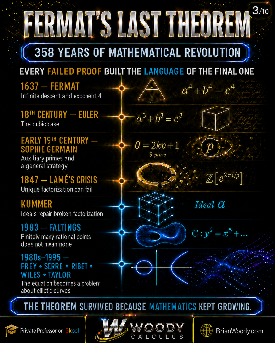
The history of Fermat’s Last Theorem is sometimes told as a 358-year collection of failed attempts followed by one triumphant proof. That version misses the mathematics.
The unsuccessful approaches were not wasted effort. Again and again, the equation exposed a weakness in the mathematical tools of the time. Mathematicians responded by inventing stronger tools:
- Fermat turned the well-ordering of the positive integers into infinite descent.
- Euler moved beyond ordinary integers toward arithmetic in larger number systems.
- Sophie Germain searched for a strategy that could control infinitely many exponents at once.
- Lamé’s proposed proof revealed that familiar factorization rules can fail in unfamiliar rings.
- Kummer repaired that failure with ideal numbers, helping create algebraic Number Theory.
- Faltings later showed that the relevant curves have only finitely many rational points, while also revealing why “finitely many” is still not “none.”
The theorem did not merely survive these ideas. It helped call them into existence.
Central historical lesson: Fermat’s Last Theorem was difficult not because mathematicians had failed to calculate far enough, but because the language required for the proof had not yet been built.
The Journey at a Glance
| Period | Mathematical advance | What it contributed |
|---|---|---|
| Around 1637 | Fermat’s marginal claim | The general problem enters mathematical history |
| Seventeenth century | Infinite descent | A proof of the fourth-power case through a smaller-solution contradiction |
| Eighteenth century | Euler and exponent \(3\) | Early movement toward arithmetic in quadratic and cyclotomic settings |
| Early nineteenth century | Sophie Germain’s auxiliary primes | The first sustained general strategy for prime exponents |
| 1825–1839 | Exponents \(5\) and \(7\) | Dirichlet, Legendre, and Lamé extend case-by-case methods |
| 1847 | The factorization crisis | A proposed general proof collapses because unique factorization cannot be assumed |
| Mid-nineteenth century | Kummer’s ideal numbers | Factorization is repaired at a deeper structural level; FLT follows for regular primes |
| 1983 | Faltings proves the Mordell conjecture | Each fixed Fermat curve of genus greater than \(1\) has finitely many rational points |
| 1980s | Frey, Serre, and Ribet | A hypothetical counterexample is translated into a non-modular elliptic curve |
| 1993–1995 | Wiles and Taylor | Semistable modularity produces the contradiction that proves FLT |
This part develops the path from Fermat through Faltings. The elliptic-curve and modular-form revolution will receive its own full treatment rather than being compressed into a few historical paragraphs.
Fermat’s Margin: What We Know and What We Do Not
Pierre de Fermat encountered a problem about Pythagorean triples while reading Claude Gaspard Bachet’s Latin translation of Diophantus’s Arithmetica. In the margin, Fermat wrote that it was impossible to separate a cube into two cubes, a fourth power into two fourth powers, or, in general, any power greater than the second into two powers of the same degree.
He then made the claim that became legendary: he had found a marvelous proof, but the margin was too narrow to contain it.
The note is conventionally dated around 1637, although the historical dating should not be treated as perfectly exact. Fermat did not publish a general proof, and no complete proof was found among his surviving papers. His son Samuel included the marginal observations in a 1670 edition of Arithmetica, bringing the claim to a wider mathematical audience.
It is tempting to turn the missing proof into a psychological mystery:
- Did Fermat possess a valid elementary proof that was later lost?
- Did he discover a proof only for a special exponent and mistakenly generalize it?
- Did he notice a flaw but never return to correct the note?
The surviving evidence cannot answer these questions conclusively. Modern mathematics strongly suggests that Fermat did not possess anything resembling the general proof ultimately found by Wiles. But “Fermat could not have known Wiles’s mathematics” is not itself a proof that no different elementary argument exists.
The responsible conclusion is narrower:
No valid general proof by Fermat survives, and the proof techniques known from his work establish only special cases—not the theorem for every exponent.
One of those special cases is extremely important. Fermat did leave an infinite-descent argument for an equivalent right-triangle result from which the exponent \(4\) case follows.
Infinite Descent: A Contradiction That Gets Smaller
Infinite descent is one of the most beautiful proof strategies in Number Theory.
The method begins by assuming that a positive-integer solution exists. Because the positive integers are well ordered, there must then be a smallest solution according to some positive-integer measure. Algebra is used to construct another solution of the same type with a strictly smaller measure.
That is impossible.
If the smallest solution produces a smaller solution, then it was never smallest. Equivalently, repeating the construction would create an infinite decreasing chain
N_1>N_2>N_3>\cdots
\]
of positive integers. No such chain exists.
This is not an argument that a sequence “approaches zero.” Nothing analytic is happening. The contradiction comes from the discrete order structure of \(\mathbb Z_{>0}\).
The descent template
- Assume at least one positive-integer solution exists.
- Choose a solution with a minimal positive-integer measure.
- Transform it into another solution of the same type.
- Prove that the new measure is strictly smaller.
- Contradict minimality.
The ingenious part is Step 3. For the fourth-power case, the Pythagorean parametrization from the opening part supplies the transformation.
Fermat’s Fourth-Power Case: A Complete Descent Proof
The following is a modernized, fully explicit version of the classical descent. It preserves the essential mechanism associated with Fermat while making every coprimality and parity step visible.
To prove Fermat’s Last Theorem for exponent \(4\), it is enough to establish a slightly stronger theorem.
Strong fourth-power theorem. There are no positive integers \(x,y,z\) satisfying \[
x^4+y^4=z^2.
\]
Why is this stronger? If a Fermat solution
x^4+y^4=w^4
\]
existed, then setting \(z=w^2\) would give
x^4+y^4=z^2.
\]
Therefore the strong theorem immediately eliminates every solution to \(x^4+y^4=w^4\).
We now prove it.
Step 1: Choose a minimal primitive solution
Assume, for contradiction, that
x^4+y^4=z^2
\]
has a positive-integer solution. Choose one with \(z\) as small as possible.
We may assume \(\gcd(x,y)=1\). If \(d=\gcd(x,y)>1\), write \(x=dX\) and \(y=dY\). Then
z^2=d^4(X^4+Y^4),
\]
so \(d^2\mid z\). Setting \(Z=z/d^2\) gives
X^4+Y^4=Z^2
\]
with \(Z<z\), contradicting the minimal choice of \(z\).
The numbers \(x\) and \(y\) cannot both be odd. Every odd fourth power is congruent to \(1\pmod{16}\), so two odd fourth powers would satisfy
x^4+y^4\equiv2\pmod{16}.
\]
But a square modulo \(16\) can only be \(0,1,4\), or \(9\), never \(2\). Because \(x\) and \(y\) are relatively prime, they also cannot both be even. Exactly one is even. Relabel if necessary so that
x\text{ is odd},
\qquad
y\text{ is even}.
\]
Step 2: Recognize a primitive Pythagorean triple
Rewrite the equation as
(x^2)^2+(y^2)^2=z^2.
\]
Thus \((x^2,y^2,z)\) is a primitive Pythagorean triple with even leg \(y^2\). The standard parametrization gives relatively prime integers \(m>n>0\) of opposite parity such that
x^2=m^2-n^2,
\qquad
y^2=2mn,
\qquad
z=m^2+n^2.
\]
The integer \(m\) must be odd and \(n\) must be even. If \(m\) were even and \(n\) odd, then
x^2=m^2-n^2\equiv-1\equiv3\pmod4,
\]
which is impossible for a square.
Write \(n=2N\). The equation \(y^2=2mn\) becomes
\left(\frac y2\right)^2=mN.
\]
Since \(\gcd(m,N)=1\) and their product is a square, both factors must be squares. Therefore there are positive integers \(u,v\) such that
m=u^2,
\qquad
N=v^2,
\qquad
n=2v^2.
\]
We have reached
x^2=u^4-4v^4.
\]
Step 3: Split a square into coprime factors
Factor the right side:
x^2=(u^2-2v^2)(u^2+2v^2).
\]
Both factors are positive and odd because \(u\) is odd. They are also relatively prime. Indeed, any common divisor would divide both their sum \(2u^2\) and their difference \(4v^2\). An odd common divisor would therefore divide both \(u\) and \(v\), contradicting \(\gcd(u,v)=1\).
We use a basic prime-factorization fact:
If two relatively prime positive integers have a product that is a square, then each integer is itself a square.
Every prime occurs in the product with an even exponent. Because the two factors share no primes, the exponent of each prime must already be even inside the factor where it occurs.
Consequently, there are positive odd integers \(r,s\), with \(s>r\), such that
r^2=u^2-2v^2,
\qquad
s^2=u^2+2v^2.
\]
Because the two squared factors are relatively prime, \(\gcd(r,s)=1\).
Subtracting gives
s^2-r^2=4v^2.
\]
Step 4: Factor again
Because \(r\) and \(s\) are odd, define
A=\frac{s+r}{2},
\qquad
B=\frac{s-r}{2}.
\]
Then \(A\) and \(B\) are positive integers, and
AB
=\frac{(s+r)(s-r)}4
=\frac{s^2-r^2}{4}
=v^2.
\]
Moreover, \(A\) and \(B\) are relatively prime. A common divisor would divide
A+B=s
\qquad\text{and}\qquad
A-B=r,
\]
but \(\gcd(r,s)=1\).
Once again, a pair of relatively prime positive integers has a square product. Therefore each factor is a square:
A=e^2,
\qquad
B=f^2
\]
for positive integers \(e,f\). It follows that
s=e^2+f^2,
\qquad
r=e^2-f^2,
\qquad
v=ef.
\]
Step 5: Construct the smaller solution
Add the equations for \(r^2\) and \(s^2\):
r^2+s^2=2u^2.
\]
Substitute \(r=e^2-f^2\) and \(s=e^2+f^2\):
\begin{aligned}
2u^2
&=(e^2-f^2)^2+(e^2+f^2)^2\\
&=2e^4+2f^4.
\end{aligned}
\]
Dividing by \(2\) gives
e^4+f^4=u^2.
\]
This is another positive-integer solution of exactly the same type as the original equation.
But it is smaller. The original right side was
z=m^2+n^2=u^4+4v^4,
\]
so certainly
0<u<z.
\]
We chose the original solution to have the smallest possible positive value of \(z\), yet it has produced a new solution whose corresponding value is \(u<z\). This is impossible.
Therefore no positive integers satisfy
x^4+y^4=z^2.
\]
In particular, no positive integers satisfy
x^4+y^4=w^4.
\]
The exponent \(4\) case of Fermat’s Last Theorem is proved.
\boxed{n=4\text{ is impossible by infinite descent.}}
\]
What made the descent work?
The proof repeatedly used three structural facts:
- Parity: fourth powers and squares occupy restricted congruence classes.
- Coprimality: when relatively prime factors multiply to a square, each factor must be a square.
- Pythagorean parametrization: a supposed fourth-power solution can be transformed into a new solution.
The contradiction is not caused by large calculations. It is caused by an impossible recursive structure: every solution would contain a smaller solution within it.
Euler and the Cubic Case
The exponent reduction from the opening part tells us that, beyond \(n=4\), the central cases are odd primes. The first is \(p=3\):
x^3+y^3=z^3.
\]
Leonhard Euler supplied the first major proof of the cubic case in the eighteenth century. As with many early arguments, the historical record deserves more nuance than the sentence “Euler proved \(n=3\).” His published treatment contained a gap in a supporting assertion, although the argument can be repaired using ideas consistent with his other work.
The cubic case already points beyond ordinary integer arithmetic. Over \(\mathbb Z\), one can factor
x^3+y^3=(x+y)(x^2-xy+y^2).
\]
An even more revealing factorization appears after introducing a primitive cube root of unity
\omega=e^{2\pi i/3},
\qquad
\omega^2+\omega+1=0.
\]
Then
x^3+y^3=(x+y)(x+\omega y)(x+\omega^2y).
\]
These factors live in the Eisenstein integers
\mathbb Z[\omega]=\{a+b\omega:a,b\in\mathbb Z\}.
\]
This ring has a workable notion of divisibility and, importantly, unique factorization. A modern proof of the cubic case can exploit that structure cleanly.
The philosophical shift is more important than the notation:
To understand an equation over the ordinary integers, it may help to factor it inside a larger number system where its hidden algebra becomes visible.
That strategy will become central. It will also create the crisis that confronted nineteenth-century mathematicians: a larger ring may permit the desired factorization without preserving unique factorization.
Sophie Germain’s Grand Strategy
For generations, Sophie Germain was treated in popular accounts as an inspiring biographical aside. Mathematically, she belongs near the center of the story.
Germain did not merely attack one exponent after another. She sought a method that could constrain broad classes of prime exponents. That ambition made her work the first sustained general program for Fermat’s Last Theorem.
The first and second cases
Let \(p\) be an odd prime, and suppose
x^p+y^p=z^p
\]
has a solution in pairwise relatively prime positive integers.
Historically, the problem is divided into two cases:
- First case: \(p\nmid xyz\). None of \(x,y,z\) is divisible by \(p\).
- Second case: \(p\mid xyz\). At least one of \(x,y,z\) is divisible by \(p\).
The second case is generally more difficult because divisibility by the exponent interacts with the factorization of the Fermat equation.
Germain’s auxiliary prime
Germain studied primes of the form
\theta=2kp+1.
\]
The prime \(\theta\) is called an auxiliary prime for the exponent \(p\) when it satisfies additional restrictions on \(p\)-th power residues modulo \(\theta\). In a standard modern formulation, the key conditions are:
- No two nonzero \(p\)-th power residues modulo \(\theta\) differ by \(1\).
- The number \(p\) is not itself a \(p\)-th power residue modulo \(\theta\).
Under these conditions, Germain’s theorem forces any hypothetical solution to have one of \(x,y,z\) divisible by \(p^2\). In particular, the first case is impossible.
This was a remarkable advance. Rather than manipulate the enormous integers \(x,y,z\) directly, Germain used modular arithmetic to restrict what their residues could do.
Concrete example: exponent \(5\)
For \(p=5\), choose
\theta=11=2(1)(5)+1.
\]
Every nonzero fifth power modulo \(11\) is congruent to \(1\) or \(-1\). Those two residues do not differ by \(1\) modulo \(11\), and \(5\) is neither \(1\) nor \(-1\pmod{11}\). Thus \(11\) satisfies the required residue conditions.
Germain’s theorem therefore eliminates the first case for exponent \(5\): any hypothetical solution would be forced into the more restrictive second case, with divisibility by \(25\).
Why the strategy was revolutionary
Germain hoped to find sufficiently many auxiliary primes to control general prime exponents. That grand plan could not be completed in the form she envisioned, but it changed the scale of the attack.
Earlier work had largely treated each exponent as its own mountain. Germain searched for a mechanism operating across an entire landscape.
Her work also illustrates a recurring principle in modern Number Theory:
A global integer equation can be attacked by studying its behavior modulo carefully chosen primes.
That local-to-global philosophy will return when elliptic curves are reduced modulo primes and their points are counted.
Dirichlet, Legendre, Lamé—and the Limits of Case-by-Case Proofs
The nineteenth century brought further victories:
- In 1825, work by Peter Gustav Lejeune Dirichlet and Adrien-Marie Legendre established the exponent \(5\) case.
- In 1839, Gabriel Lamé proved the exponent \(7\) case.
These were serious achievements. They also made a strategic weakness increasingly visible.
The proof for \(p=3\) did not automatically prove \(p=5\). The proof for \(p=5\) did not automatically prove \(p=7\). As the exponent increased, the algebra became more complicated. Even if mathematicians proved a thousand individual exponents, infinitely many primes would remain.
The problem needed a theory capable of treating the exponent \(p\) symbolically.
Cyclotomic factorization appeared to offer exactly that.
The 1847 Crisis: A Beautiful Proof That Did Not Work
Let \(p\) be an odd prime, and let
\zeta_p=e^{2\pi i/p}
\]
be a primitive \(p\)-th root of unity. In the cyclotomic ring
\mathbb Z[\zeta_p],
\]
the left side of Fermat’s equation factors completely:
x^p+y^p
=\prod_{j=0}^{p-1}(x+\zeta_p^j y).
\]
This looks like the decisive move. The single equation has split into \(p\) linear factors. If the factors are sufficiently coprime and their product is a \(p\)-th power, one would like to conclude that each factor is essentially a \(p\)-th power. From there, a contradiction might follow.
In 1847, Lamé announced to the French Academy of Sciences that this approach produced a general proof. The announcement created immediate excitement—and immediate scrutiny.
The hidden assumption was unique factorization.
Lamé’s reasoning treated \(\mathbb Z[\zeta_p]\) as though every element factored uniquely into irreducibles, just as every positive integer factors uniquely into ordinary primes. That property cannot be taken for granted. For many cyclotomic rings, it is false.
Why unique factorization matters
In \(\mathbb Z\), suppose relatively prime integers \(A\) and \(B\) satisfy
AB=C^p.
\]
Unique prime factorization tells us that every prime exponent in \(A\) and \(B\) must be divisible by \(p\). Therefore \(A\) and \(B\) are each \(p\)-th powers, up to units.
That inference powered the descent proof earlier in this lesson when \(p=2\).
Without unique factorization, the conclusion can fail. An element may admit genuinely different decompositions into irreducibles, so reading divisibility information from a displayed product becomes unsafe.
The familiar example
6=2\cdot3=(1+\sqrt{-5})(1-\sqrt{-5})
\]
in the ring \(\mathbb Z[\sqrt{-5}]\) shows the phenomenon. The displayed factors are irreducible in that ring, yet the two factorizations are not equivalent through reordering and multiplication by units.
This example is not the cyclotomic ring from Fermat’s equation. It is a simpler warning: algebraic integers need not obey the factorization rules of \(\mathbb Z\).
The failure was productive
Lamé’s proof could not be repaired by inserting one missing calculation. The failure exposed a structural problem:
\boxed{\text{Elements may fail to factor uniquely in rings of algebraic integers.}}
\]
The next breakthrough required mathematicians to change what they meant by a factor.
Kummer’s Ideal Numbers: Repairing Factorization
Ernst Eduard Kummer had already been investigating the arithmetic of cyclotomic integers. He understood that unique factorization of elements could fail and developed a replacement: ideal numbers.
The modern language of ideals was later formalized and generalized by Richard Dedekind. From that perspective, the central repair is:
Elements may not factor uniquely, but nonzero ideals in the ring of integers of a number field do factor uniquely into prime ideals.
This is one of the great conceptual upgrades in algebra.
From elements to ideals
In an ordinary principal ideal domain, an element \(\alpha\) and the principal ideal it generates,
(\alpha)=\{r\alpha:r\in R\},
\]
carry essentially the same divisibility information.
In a more general ring of algebraic integers, a nonprincipal ideal may behave like a “missing factor” that cannot be represented by a single element. By enlarging the factorization theory from elements to ideals, these hidden factors become visible.
The obstruction to every ideal being principal is measured by the ideal class group. Its size is the class number.
- Class number \(1\): every ideal is principal, and the ring has unique factorization of elements.
- Class number greater than \(1\): nonprincipal ideals exist, so element factorization can fail even though ideal factorization remains unique.
The distinction between element factorization and ideal factorization is exactly the distinction Lamé’s proposed proof had overlooked.
Regular primes
For an odd prime \(p\), consider the cyclotomic field
\mathbb Q(\zeta_p).
\]
The prime \(p\) is called regular if it does not divide the class number of this field. Kummer found an equivalent criterion involving Bernoulli numbers: \(p\) is regular precisely when it does not divide the numerator of any of
B_2,B_4,B_6,\ldots,B_{p-3}.
\]
Kummer proved Fermat’s Last Theorem for every regular prime exponent.
All odd primes below \(37\) are regular. The first irregular prime is
37,
\]
which divides the numerator of \(B_{32}\).
Kummer’s theorem therefore covered a vast family of exponents and explained why certain prime exponents were more difficult than others. But irregular primes remained, so the general theorem was still open.
Why Kummer’s “failure to finish” was a triumph
Judged only by the final yes-or-no question, Kummer did not prove Fermat’s Last Theorem for every exponent. Judged mathematically, his work was transformative.
The attempt to factor Fermat’s equation led to:
- cyclotomic fields,
- ideal numbers and later ideals,
- class groups and class numbers,
- regular and irregular primes,
- deep connections with Bernoulli numbers.
The equation had forced mathematics to distinguish between the arithmetic of elements and the arithmetic of ideals.
This is why Fermat’s Last Theorem matters beyond its final statement. Even before it was proved, it was functioning as a machine for generating mathematics.
Faltings: Why “Finitely Many” Is Not “None”
By the twentieth century, Fermat’s equation could also be viewed geometrically. For a fixed exponent \(n\), consider the projective Fermat curve
X^n+Y^n=Z^n.
\]
For \(n\ge4\), this smooth projective curve has genus
g=\frac{(n-1)(n-2)}2>1.
\]
In 1983, Gerd Faltings proved the Mordell conjecture: a smooth projective curve of genus greater than \(1\) over a number field has only finitely many rational points.
Applied to a fixed Fermat curve with \(n\ge4\), Faltings’s theorem gives:
\boxed{X^n+Y^n=Z^n\text{ has only finitely many rational projective points.}}
\]
This is an astonishing finiteness theorem. Yet it does not prove Fermat’s Last Theorem.
Finite does not mean zero
A finite set may contain no elements, one element, or millions of elements. Faltings’s theorem says the set is finite; it does not list the points or declare that every nontrivial point is absent.
The Fermat curve always has trivial rational points with a zero coordinate, such as
[1:0:1]
\qquad\text{and}\qquad
[0:1:1].
\]
Fermat’s Last Theorem asks whether any nontrivial rational point exists with \(XYZ\ne0\). Faltings gives finiteness but does not, by itself, separate the trivial points from hypothetical nontrivial ones.
The cubic Fermat curve \(n=3\) has genus \(1\), so it does not fall under the genus-greater-than-one statement of Faltings’s theorem. Its case had already been settled separately.
This distinction is essential:
\text{Faltings: finitely many rational points for each fixed }n\ge4.
\]
\text{Fermat: no nontrivial rational points for every }n>2.
\]
The first does not automatically imply the second.
The problem still needed a bridge
Faltings showed that the rational points on each high-degree Fermat curve are severely constrained. But Fermat’s Last Theorem needed a mechanism that would eliminate a hypothetical nontrivial point entirely.
That mechanism arrived from an unexpected direction. Instead of studying the Fermat curve alone, mathematicians learned to use a supposed Fermat solution to construct a different curve—an elliptic curve.
What the First 346 Years Accomplished
By the early 1980s, the theorem remained unproved, but the mathematical landscape had been transformed.
Fermat contributed a proof architecture
Infinite descent showed how a positive-integer solution could be destroyed by extracting a smaller copy of itself.
Euler revealed the value of enlarged number systems
The cubic case demonstrated that roots of unity and new rings could expose factorizations invisible in \(\mathbb Z\).
Germain contributed a general strategy
Auxiliary primes showed how modular restrictions could control hypothetical global solutions across families of exponents.
Kummer replaced broken elements with ideals
Unique factorization returned at the ideal level, and the obstruction was encoded by the class group.
Faltings imposed geometric finiteness
For each fixed exponent \(n\ge4\), the relevant Fermat curve has only finitely many rational points.
None of these ideas was the final proof. All of them changed what a final proof could look like.
Then came the conceptual leap:
If a Fermat counterexample existed, perhaps the most revealing object would not be the integers \(a,b,c\) or even the Fermat curve itself, but an elliptic curve manufactured from the supposed solution.
That is the Frey curve, and it changes the story completely.
Part III — Elliptic Curves and the Birth of the Frey Curve
For more than three centuries, mathematicians attacked Fermat’s equation through integers, congruences, factorizations, and algebraic number fields. Then the problem changed shape.
Suppose, only for the sake of contradiction, that positive integers satisfy
a^p+b^p=c^p
\]
for some prime \(p\ge5\). Instead of trying to manipulate those powers until they collapse, we use them to build a new object:
E_{a,b,p}:\quad y^2=x(x-a^p)(x+b^p).
\]
This is the Frey–Hellegouarch curve. It converts a hypothetical solution of Fermat’s equation into an elliptic curve with an extraordinarily rigid arithmetic fingerprint.
The change of viewpoint is radical:
\boxed{
\text{A forbidden equation in integers}
\quad\longrightarrow\quad
\text{a hypothetical elliptic curve.}
}
\]
Ribet and Wiles will eventually force incompatible conclusions about this curve. Before that argument can mean anything, we need to understand what an elliptic curve is, why its points form a group, what happens over a finite field, and exactly how the Fermat powers become encoded in its discriminant.
What Is an Elliptic Curve?
An elliptic curve is not an ellipse.
Over a field whose characteristic is not \(2\) or \(3\), an elliptic curve can be written in short Weierstrass form as
E:\quad y^2=x^3+Ax+B,
\]
where
4A^3+27B^2\ne0.
\]
It also includes a distinguished point at infinity, denoted by \(\mathcal O\).
The complete abstract definition is a nonsingular projective curve of genus \(1\) together with a specified base point. The Weierstrass equation gives us a concrete model on which we can calculate.
Why “elliptic” if it is not an ellipse?
The name comes historically from elliptic integrals, which arose in questions such as computing the arc length of an ellipse. Inverting those integrals led to elliptic functions, and elliptic curves became the algebraic objects underlying that theory.
The word describes the history of the mathematics, not the visible shape of the graph.
The discriminant condition
For
y^2=x^3+Ax+B,
\]
the discriminant is
\Delta=-16(4A^3+27B^2).
\]
The condition \(\Delta\ne0\) means the cubic on the right has no repeated root. Geometrically, the curve has no cusp, crossing, or other singular point.
If \(\Delta=0\), the equation may still draw a curve, but it is not an elliptic curve. For example,
y^2=x^3
\]
has a cusp at \((0,0)\), while
y^2=x^2(x+1)
\]
has a singular point at the origin.
Nonsingularity is not a cosmetic preference. The group law depends on it.
The Same Equation Over Different Fields
An elliptic curve is defined over a field, and the field determines which points are available.
Consider
E:\quad y^2=x^3-x+1.
\]
Its discriminant is
\Delta=-16\bigl(4(-1)^3+27(1)^2\bigr)
=-16(23)
=-368\ne0.
\]
So this is a nonsingular elliptic curve over \(\mathbb Q\).
We can study several different point sets:
- \(E(\mathbb R)\): points whose coordinates are real numbers.
- \(E(\mathbb Q)\): points whose coordinates are rational numbers.
- \(E(\mathbb C)\): points whose coordinates are complex numbers.
- \(E(\mathbb F_q)\): points over a finite field with \(q\) elements.
These are not different equations. They are different arithmetic worlds in which the same equation is interpreted.
The real points form a smooth geometric curve. The rational points are a generally sparse subset of that curve. Over a finite field, the “curve” becomes a finite collection of points.
The point at infinity
The affine equation does not visibly contain \(\mathcal O\). It appears when the curve is placed in the projective plane.
Homogenizing the equation gives
Y^2Z=X^3+AXZ^2+BZ^3.
\]
Setting \(Z=0\) produces the unique projective point
\mathcal O=[0:1:0].
\]
This point will act as the identity element of the elliptic-curve group.
Why Elliptic-Curve Points Can Be Added
The extraordinary feature of an elliptic curve is that its points can be added.
Let \(P\) and \(Q\) be two points on a nonsingular cubic. A line through \(P\) and \(Q\) usually meets the cubic at exactly one additional point \(R\), counting multiplicity. Reflect \(R\) across the \(x\)-axis. The reflected point is defined to be
P+Q.
\]
This is the chord-and-tangent law.
If \(P=Q\), use the tangent line at \(P\) instead of a chord. If the line through \(P\) and \(Q\) is vertical, its third intersection is the point at infinity, so
P+(-P)=\mathcal O.
\]
The picture motivates the operation. Algebra makes it exact.
Addition formulas
Let
E:\quad y^2=x^3+Ax+B.
\]
For distinct points
P=(x_1,y_1),
\qquad
Q=(x_2,y_2),
\qquad
x_1\ne x_2,
\]
define the slope
\lambda=\frac{y_2-y_1}{x_2-x_1}.
\]
Then \(P+Q=(x_3,y_3)\), where
x_3=\lambda^2-x_1-x_2
\]
and
y_3=\lambda(x_1-x_3)-y_1.
\]
For doubling \(P=(x_1,y_1)\) with \(y_1\ne0\), the tangent slope is
\lambda=\frac{3x_1^2+A}{2y_1},
\]
followed by the same coordinate formulas:
x_{2P}=\lambda^2-2x_1,
\qquad
y_{2P}=\lambda(x_1-x_{2P})-y_1.
\]
The inverse of \(P=(x,y)\) is
-P=(x,-y).
\]
If \(y=0\), then \(P=-P\), so
2P=\mathcal O.
\]
Worked Addition Over \(\mathbb Q\)
Return to
E:\quad y^2=x^3-x+1.
\]
Choose
P=(0,1),
\qquad
Q=(1,1).
\]
Both points lie on the curve:
1^2=0^3-0+1
\]
and
1^2=1^3-1+1.
\]
Geometric calculation of \(P+Q\)
The line through \(P\) and \(Q\) is horizontal:
y=1.
\]
Substitute into the curve:
1=x^3-x+1.
\]
Therefore
x^3-x=x(x-1)(x+1)=0.
\]
The three intersections occur at \(x=0,1,-1\). The first two are \(P\) and \(Q\), so the third is
R=(-1,1).
\]
Reflecting across the \(x\)-axis gives
\boxed{P+Q=(-1,-1).}
\]
Algebraic verification
The slope is
\lambda=\frac{1-1}{1-0}=0.
\]
Then
x_3=0^2-0-1=-1
\]
and
y_3=0(0-(-1))-1=-1.
\]
The geometric and algebraic calculations agree.
Worked Doubling Over \(\mathbb Q\)
Now calculate \(2P\) for
P=(0,1).
\]
The tangent slope is
\lambda
=\frac{3(0)^2-1}{2(1)}
=-\frac12.
\]
Therefore
x_{2P}
=\left(-\frac12\right)^2-2(0)
=\frac14.
\]
The \(y\)-coordinate is
\begin{aligned}
y_{2P}
&=-\frac12\left(0-\frac14\right)-1\\
&=\frac18-1\\
&=-\frac78.
\end{aligned}
\]
Thus
\boxed{2P=\left(\frac14,-\frac78\right).}
\]
Verify the result directly:
\left(-\frac78\right)^2=\frac{49}{64}
\]
and
\left(\frac14\right)^3-\frac14+1
=\frac1{64}-\frac{16}{64}+\frac{64}{64}
=\frac{49}{64}.
\]
The doubled point lies on the curve.
The Elliptic-Curve Group
With this addition law, the points form an abelian group:
- Closure: \(P+Q\) is another point on the curve.
- Identity: \(P+\mathcal O=P\).
- Inverse: \(P+(-P)=\mathcal O\).
- Commutativity: \(P+Q=Q+P\).
- Associativity: \((P+Q)+R=P+(Q+R)\).
The geometry makes closure, inverses, and commutativity plausible. Associativity is the subtle axiom. A picture alone does not prove it; the result follows from the algebraic geometry of the cubic or from a direct but lengthy verification of the formulas.
For a curve over \(\mathbb Q\), Mordell’s theorem states that the rational-point group is finitely generated:
E(\mathbb Q)\cong E(\mathbb Q)_{\mathrm{tors}}\oplus\mathbb Z^r.
\]
Here:
- \(E(\mathbb Q)_{\mathrm{tors}}\) is a finite torsion subgroup.
- \(r\) is the rank.
- A positive rank produces infinitely many rational points by repeatedly adding independent points.
The group law converts geometry into arithmetic. Points can now carry divisibility, torsion, generation, and representation-theoretic information.
Elliptic Curves Over Finite Fields
Now interpret the same curve modulo a prime.
Let
E:\quad y^2=x^3-x+1
\]
over the finite field
\mathbb F_5=\{0,1,2,3,4\}.
\]
All arithmetic is performed modulo \(5\). The possible square residues are
0^2\equiv0,
\qquad
1^2\equiv4^2\equiv1,
\qquad
2^2\equiv3^2\equiv4
\pmod5.
\]
For each \(x\), compute \(x^3-x+1\pmod5\):
| \(x\) | \(x^3-x+1\pmod5\) | Solutions for \(y\) |
|---|---|---|
| \(0\) | \(1\) | \(y=1,4\) |
| \(1\) | \(1\) | \(y=1,4\) |
| \(2\) | \(2\) | none |
| \(3\) | \(0\) | \(y=0\) |
| \(4\) | \(1\) | \(y=1,4\) |
Including the point at infinity, we obtain
\begin{aligned}
E(\mathbb F_5)=\{&\mathcal O,
(0,1),(0,4),
(1,1),(1,4),\\
&(3,0),(4,1),(4,4)\}.
\end{aligned}
\]
Therefore
\boxed{\#E(\mathbb F_5)=8.}
\]
The continuous real curve has become a finite eight-element group.
Division in a finite field
The addition formulas still work, but division means multiplying by a modular inverse.
For example,
2^{-1}\equiv3\pmod5
\]
because
2\cdot3\equiv1\pmod5.
\]
Every nonzero element of \(\mathbb F_5\) has a multiplicative inverse, which is exactly why the formulas make sense whenever their denominators are nonzero.
Worked Addition Over \(\mathbb F_5\)
Use the same coordinate points
P=(0,1),
\qquad
Q=(1,1).
\]
The slope is
\lambda=\frac{1-1}{1-0}=0.
\]
Then
x_3\equiv0^2-0-1\equiv4\pmod5
\]
and
y_3\equiv0(0-4)-1\equiv4\pmod5.
\]
Thus
\boxed{P+Q=(4,4)\text{ in }E(\mathbb F_5).}
\]
This is precisely the reduction modulo \(5\) of the rational result
P+Q=(-1,-1),
\]
because \(-1\equiv4\pmod5\).
Doubling modulo \(5\)
For \(P=(0,1)\),
\lambda
\equiv\frac{-1}{2}
\equiv(-1)(3)
\equiv2
\pmod5.
\]
Therefore
x_{2P}\equiv2^2-0\equiv4\pmod5
\]
and
y_{2P}
\equiv2(0-4)-1
\equiv-9
\equiv1
\pmod5.
\]
Hence
\boxed{2P=(4,1).}
\]
Continuing to add \(P\) generates every point in the group:
\begin{array}{c|c}
k & kP\\
\hline
1&(0,1)\\
2&(4,1)\\
3&(1,4)\\
4&(3,0)\\
5&(1,1)\\
6&(4,4)\\
7&(0,4)\\
8&\mathcal O
\end{array}
\]
Thus \(P\) has order \(8\), and in this example
E(\mathbb F_5)\cong\mathbb Z/8\mathbb Z.
\]
This finite-group structure is the mathematical foundation used by elliptic-curve cryptography. Cryptographic systems use enormously larger finite fields, but the underlying operations are still point addition and repeated doubling.
Point Counts as an Arithmetic Fingerprint
For a prime \(\ell\) at which an elliptic curve has good reduction, define
a_\ell(E)=\ell+1-\#E(\mathbb F_\ell).
\]
For our example at \(\ell=5\),
a_5(E)=5+1-8=-2.
\]
This is a good prime because
5\nmid\Delta=-368.
\]
The Hasse bound states
|a_\ell(E)|\le2\sqrt\ell.
\]
Here
|-2|=2\le2\sqrt5.
\]
One point count is only one piece of data. Repeating the calculation across all good primes produces a sequence
a_3(E),a_5(E),a_7(E),a_{11}(E),\ldots
\]
for this particular curve, with its primes of bad reduction omitted or treated separately. This sequence acts like an arithmetic barcode for the elliptic curve.
In the next part, modular forms will produce their own coefficient sequence
a_1(f),a_2(f),a_3(f),\ldots
\]
Modularity means that the two arithmetic fingerprints match at every good prime:
a_\ell(E)=a_\ell(f).
\]
This is the first concrete glimpse of the bridge Wiles needed.
From a Hypothetical Fermat Solution to the Frey Curve
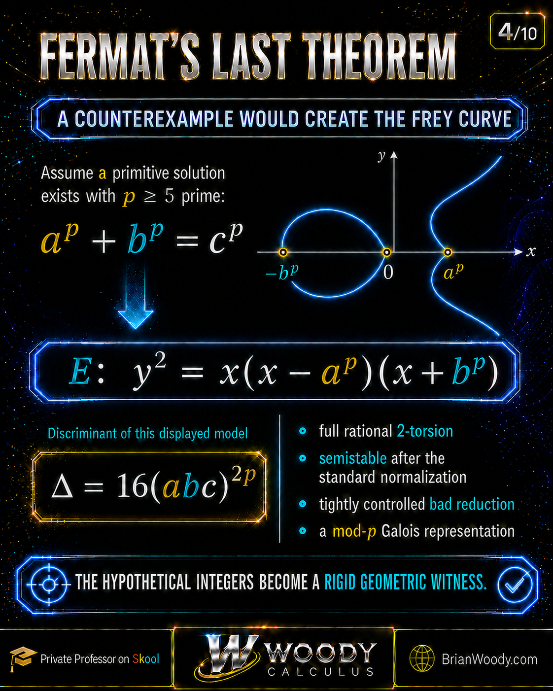
We now return to Fermat’s Last Theorem.
Assume, toward a contradiction, that there is a primitive solution
a^p+b^p=c^p,
\qquad
p\ge5\text{ prime},
\qquad
\gcd(a,b,c)=1.
\]
After interchanging \(a\) and \(b\) if necessary and applying the standard parity normalization, attach the curve
\boxed{
E_{a,b,p}:\quad y^2=x(x-a^p)(x+b^p).
}
\]
This is a hypothetical curve in the FLT argument. We do not have numerical values of \(a,b,c,p\), because Fermat’s Last Theorem says no such values exist. The curve is constructed inside a proof by contradiction.
Why this equation defines an elliptic curve
Set
A=a^p,
\qquad
B=b^p,
\qquad
C=c^p=A+B.
\]
The cubic is
x(x-A)(x+B).
\]
Its three roots are
0,
\qquad
A,
\qquad
-B.
\]
They are distinct because \(A,B,C\) are nonzero and
A-(-B)=A+B=C\ne0.
\]
Therefore the cubic has no repeated root, so the curve is nonsingular over \(\mathbb Q\). It is a legitimate elliptic curve.
The roots also give three visible rational points of order \(2\):
(0,0),
\qquad
(A,0),
\qquad
(-B,0).
\]
Each point equals its own inverse because its \(y\)-coordinate is zero.
Deriving the Frey Curve’s Discriminant
For a cubic written as
y^2=(x-e_1)(x-e_2)(x-e_3),
\]
the Weierstrass discriminant is
\Delta=16(e_1-e_2)^2(e_1-e_3)^2(e_2-e_3)^2.
\]
For the Frey curve,
e_1=0,
\qquad
e_2=A,
\qquad
e_3=-B.
\]
The three root differences are, up to sign,
A,
\qquad
B,
\qquad
A+B=C.
\]
Therefore
\begin{aligned}
\Delta
&=16A^2B^2C^2\\
&=16(a^p)^2(b^p)^2(c^p)^2\\
&=16(abc)^{2p}.
\end{aligned}
\]
Thus
\boxed{\Delta=16(abc)^{2p}.}
\]
The discriminant is not merely large. Away from the factor \(16\), it is a perfect \(2p\)-th power. The supposed Fermat solution has been embedded directly into the arithmetic of the curve.
This is one reason the Frey curve is so powerful: the original Diophantine equation controls the primes of bad reduction and the valuations appearing in the discriminant.
Good, Multiplicative, and Additive Reduction
An elliptic curve over \(\mathbb Q\) can be reduced modulo a prime \(\ell\) by reducing the coefficients of an integral model modulo \(\ell\).
Three broad behaviors can occur:
- Good reduction: the reduced curve remains nonsingular.
- Multiplicative reduction: the reduced cubic acquires a node.
- Additive reduction: the reduction becomes more severely singular, such as developing a cusp.
An elliptic curve is semistable if every prime has either good or multiplicative reduction—never additive reduction.
For the properly normalized Frey curve arising from a primitive hypothetical Fermat solution, local analysis shows that the curve is semistable.
The displayed discriminant tells us where bad reduction can occur: only primes dividing
2abc.
\]
However, the exact minimal discriminant and conductor require prime-by-prime changes of variables and careful treatment of parity, especially at \(2\). We will not replace that analysis with an oversimplified conductor formula.
The safe conclusion needed for the proof is:
\boxed{
\text{A primitive Fermat counterexample with }p\ge5
\text{ would produce a semistable elliptic curve over }\mathbb Q.
}
\]
This word—semistable—is exactly what brings the curve inside the theorem Wiles ultimately proved.
Why the Frey Curve Is the Perfect Carrier
The Frey curve packages several decisive properties into one object.
It remembers the Fermat equation
The root difference
a^p-(-b^p)=a^p+b^p=c^p
\]
is precisely the Fermat relation.
It has controlled bad reduction
The discriminant
16(abc)^{2p}
\]
concentrates bad reduction at primes dividing \(2abc\), with unusually large exponents tied to \(p\).
It is semistable
This places it in the exact class of elliptic curves covered by the Wiles–Taylor semistable modularity theorem.
It has a mod-\(p\) Galois representation
The Galois group of \(\mathbb Q\) acts on the \(p\)-torsion points of the curve, producing
\bar\rho_{E,p}:
\operatorname{Gal}(\overline{\mathbb Q}/\mathbb Q)
\longrightarrow
\operatorname{GL}_2(\mathbb F_p).
\]
This representation carries enough arithmetic information for Ribet’s level-lowering theorem to act on it.
It enters two incompatible theorems
Ribet’s theorem implies that a Frey curve arising from an FLT counterexample cannot be modular. Wiles–Taylor implies that every semistable elliptic curve over \(\mathbb Q\) is modular.
The curve is not impossible because its graph looks strange. It is impossible because its arithmetic properties force a logical contradiction.
The Proof Map After the Frey Curve
We can now expand the first arrow in the modern proof:
\begin{aligned}
&a^p+b^p=c^p
\quad(p\ge5,\text{ primitive hypothetical solution})\\[4pt]
&\Downarrow\\[4pt]
&E_{a,b,p}:y^2=x(x-a^p)(x+b^p)\\[4pt]
&\Downarrow\\[4pt]
&\Delta=16(abc)^{2p},
\quad E_{a,b,p}\text{ semistable}\\[4pt]
&\Downarrow\\[4pt]
&\text{Ribet: }E_{a,b,p}\text{ cannot be modular}\\[4pt]
&\text{Wiles–Taylor: }E_{a,b,p}\text{ must be modular}\\[4pt]
&\Downarrow\\[4pt]
&\text{Contradiction.}
\end{aligned}
\]
We now understand what the curve is and why the Fermat equation is visible inside it. The next task is to understand what modular means.
Part IV — Modular Forms and Arithmetic Fingerprints
The preceding elliptic-curve part produced an elliptic curve from a hypothetical Fermat counterexample. The modern proof now asks a question that would have sounded astonishing to a nineteenth-century number theorist:
Does this cubic curve come from a highly symmetric analytic function on the complex upper half-plane?
That is the question of modularity.
An elliptic curve is an algebraic and geometric object. A modular form is a complex analytic function obeying rigid transformation laws. They do not look alike, live in the same space, or use the same defining equations.
Yet both objects generate sequences of arithmetic numbers.
For an elliptic curve \(E/\mathbb Q\), count points modulo primes:
a_\ell(E)=\ell+1-\#E(\mathbb F_\ell).
\]
For a modular form, read the coefficients of its \(q\)-expansion:
f(z)=\sum_{n=0}^{\infty}a_n(f)q^n,
\qquad
q=e^{2\pi iz}.
\]
The Modularity Theorem says that every elliptic curve over \(\mathbb Q\) has a matching weight-two newform. At every prime of good reduction,
\boxed{a_\ell(E)=a_\ell(f).}
\]
The two objects share the same arithmetic fingerprint.
That equality is not an analogy. In this part, we verify it numerically for the exact elliptic curve introduced above.
The Complex Upper Half-Plane
Modular forms live on the complex upper half-plane
\mathbb H
=\{z\in\mathbb C:\operatorname{Im}(z)>0\}.
\]
Write
z=x+iy,
\qquad
y>0.
\]
The group
\operatorname{SL}_2(\mathbb Z)
=\left\{
\begin{pmatrix}a&b\\c&d\end{pmatrix}
:a,b,c,d\in\mathbb Z,
\ ad-bc=1
\right\}
\]
acts on \(\mathbb H\) by fractional-linear transformations:
\gamma z
=\frac{az+b}{cz+d},
\qquad
\gamma=
\begin{pmatrix}a&b\\c&d\end{pmatrix}.
\]
This action preserves the upper half-plane because
\operatorname{Im}(\gamma z)
=\frac{\operatorname{Im}(z)}{|cz+d|^2}>0.
\]
Two especially important transformations are
T:z\longmapsto z+1
\]
and
S:z\longmapsto-\frac1z.
\]
These generate the modular group up to its center. A modular form is constrained by transformations of this kind.
Why this is deeper than ordinary periodicity
A periodic function may satisfy
f(z+1)=f(z).
\]
A modular form satisfies periodicity and an inversion-type symmetry, together with all the relations generated by the relevant matrix group. These symmetries tie values of the function at distant points of \(\mathbb H\) to one another.
That rigidity is what allows analytic functions to encode arithmetic.
Level and the Congruence Subgroup \(\Gamma_0(N)\)
Elliptic curves are matched with modular forms on specific congruence subgroups.
For a positive integer \(N\), define
\Gamma_0(N)
=\left\{
\begin{pmatrix}a&b\\c&d\end{pmatrix}
\in\operatorname{SL}_2(\mathbb Z)
:c\equiv0\pmod N
\right\}.
\]
The integer \(N\) is called the level.
The matrix
T=
\begin{pmatrix}1&1\\0&1\end{pmatrix}
\]
belongs to every \(\Gamma_0(N)\), so modular forms of level \(N\) remain periodic under \(z\mapsto z+1\).
When a modular form corresponds to an elliptic curve, its level equals the conductor of the curve. The conductor compresses the curve’s bad-reduction behavior into one integer.
This equality
\boxed{\text{level of }f=\text{conductor of }E}
\]
is one of the precise ways the analytic and algebraic sides align.
What Is a Modular Form?
Let \(k\) be a nonnegative integer. A modular form of weight \(k\) and level \(N\), with trivial character, is a holomorphic function
f:\mathbb H\longrightarrow\mathbb C
\]
satisfying
f\!\left(\frac{az+b}{cz+d}\right)
=(cz+d)^k f(z)
\]
for every
\begin{pmatrix}a&b\\c&d\end{pmatrix}
\in\Gamma_0(N),
\]
together with a holomorphicity condition at every cusp.
More general modular forms may include a Dirichlet character in the transformation law. The newform associated with our worked elliptic curve has trivial character, so the displayed version is the one we need.
What does weight mean?
The exponent \(k\) controls how the function changes under a fractional-linear transformation. A weight-zero modular function would be invariant. A positive-weight modular form transforms by the factor
(cz+d)^k.
\]
Elliptic curves over \(\mathbb Q\) correspond to modular forms of weight
\boxed{k=2.}
\]
This specific weight is not arbitrary. Weight-two cusp forms behave like holomorphic differentials on modular curves, making them the correct analytic objects to connect with elliptic curves.
What is a cusp?
The upper half-plane is enlarged by certain rational boundary points and the point \(i\infty\). These boundary classes are called cusps.
As \(\operatorname{Im}(z)\to\infty\), we have
q=e^{2\pi iz}\longrightarrow0.
\]
Holomorphicity at the cusp \(i\infty\) becomes a condition on the powers of \(q\) appearing in the Fourier expansion. The definition requires corresponding regularity at every cusp, not only at infinity.
Why Modular Forms Have \(q\)-Expansions
Since
f(z+1)=f(z),
\]
the function is periodic with period \(1\). It therefore has a Fourier expansion. With
q=e^{2\pi iz},
\]
we write
f(z)=\sum_{n=0}^{\infty}a_nq^n.
\]
Holomorphicity at \(i\infty\) rules out negative powers of \(q\).
A cusp form vanishes at every cusp. At \(i\infty\), this forces
a_0=0,
\]
so its expansion begins
f(z)=a_1q+a_2q^2+a_3q^3+\cdots.
\]
A cusp form is normalized when
a_1=1.
\]
The coefficients are not decorative Fourier data. For Hecke eigenforms, they satisfy strong multiplicative laws and encode information about primes.
First Example: Ramanujan’s Delta Function
A famous normalized cusp form is the Ramanujan discriminant modular form
\Delta_{\mathrm{Ram}}(z)
=q\prod_{n=1}^{\infty}(1-q^n)^{24}.
\]
Its expansion begins
\Delta_{\mathrm{Ram}}(z)
=q-24q^2+252q^3-1472q^4+4830q^5-\cdots.
\]
These coefficients are the values of the famous Ramanujan tau function:
\Delta_{\mathrm{Ram}}(z)
=\sum_{n=1}^{\infty}\tau(n)q^n.
\]
Thus \(\tau(1)=1\), \(\tau(2)=-24\), \(\tau(3)=252\), and so on.
It is a weight-\(12\), level-\(1\) cusp form:
\Delta_{\mathrm{Ram}}\!\left(\frac{az+b}{cz+d}\right)
=(cz+d)^{12}\Delta_{\mathrm{Ram}}(z)
\]
for matrices in \(\operatorname{SL}_2(\mathbb Z)\).
The notation \(\Delta_{\mathrm{Ram}}\) should not be confused with the discriminant \(\Delta(E)\) of an elliptic curve. They are different objects sharing a traditional symbol.
Ramanujan’s form is a perfect introduction to \(q\)-expansions, but it is not the modular form attached to an elliptic curve over \(\mathbb Q\): its weight is \(12\), not \(2\).
To see elliptic-curve modularity, we need a weight-two newform.
Hecke Operators: Why the Coefficients Behave Like Arithmetic
For fixed weight and level, modular forms form finite-dimensional complex vector spaces. Hecke operators are commuting linear transformations acting on those spaces.
A Hecke eigenform is a simultaneous eigenvector for the Hecke operators. For a normalized eigenform
f(z)=\sum_{n=1}^{\infty}a_nq^n,
\]
the coefficient \(a_n\) is the corresponding Hecke eigenvalue, with the usual operator conventions at primes dividing the level.
The eigenform property forces multiplicativity. For relatively prime positive integers \(m,n\),
a_{mn}=a_ma_n.
\]
For a prime \(\ell\nmid N\), the prime-power coefficients satisfy
a_{\ell^r}
=a_\ell a_{\ell^{r-1}}
-\ell^{k-1}a_{\ell^{r-2}}.
\]
In weight \(2\), this becomes
a_{\ell^r}
=a_\ell a_{\ell^{r-1}}
-\ell a_{\ell^{r-2}}.
\]
These relations show that the prime-indexed coefficients control the rest of the expansion.
What is a newform?
At level \(N\), some cusp forms are inherited from lower levels. These are called oldforms. A newform is a normalized Hecke eigenform belonging to the genuinely new part of level \(N\).
The primitive arithmetic information at level \(N\) lives in its newforms.
Elliptic curves over \(\mathbb Q\) correspond to normalized weight-two newforms with rational coefficients.
Our Verified Elliptic Curve and Its Newform
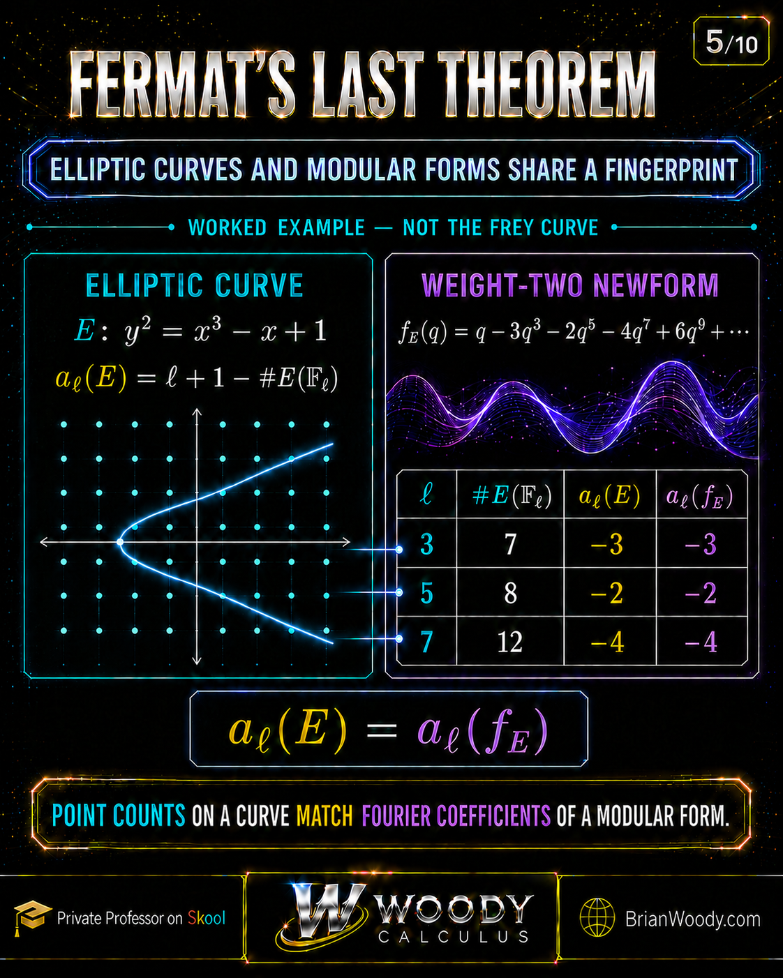
The elliptic-curve part used the curve
E:\quad y^2=x^3-x+1.
\]
Its minimal discriminant and conductor are
\Delta(E)=-368=-2^4\cdot23
\]
and
N_E=92=2^2\cdot23.
\]
In standard database notation, the curve has LMFDB label
92.a1
\]
and Cremona label \(92b1\).
Its corresponding normalized weight-two newform has level \(92\) and label
92.2.a.a.
\]
The \(q\)-expansion begins
\begin{aligned}
f_E(z)
=\;&q-3q^3-2q^5-4q^7+6q^9+2q^{11}\\
&-5q^{13}+6q^{15}+4q^{17}-2q^{19}+O(q^{20}).
\end{aligned}
\]
Coefficients not displayed in this range are zero. In particular,
a_2=0.
\]
That zero reflects additive reduction at \(2\). The curve also has split multiplicative reduction at \(23\). Therefore this particular example is not semistable.
That distinction is useful:
- The full Modularity Theorem guarantees that this curve is modular.
- Wiles’s original theorem established the semistable case.
- The hypothetical Frey curve is semistable, so Wiles’s result is exactly strong enough for Fermat’s Last Theorem.
We must not use the modern modularity of our nonsemistable example to misstate the historical scope of Wiles’s 1995 theorem.
Recompute the First Match by Hand
Take the good prime
\ell=3.
\]
Reduce the curve modulo \(3\):
y^2\equiv x^3-x+1\pmod3.
\]
The square residues modulo \(3\) are \(0\) and \(1\). Evaluate the right side:
| \(x\) | \(x^3-x+1\pmod3\) | Values of \(y\) |
|---|---|---|
| \(0\) | \(1\) | \(1,2\) |
| \(1\) | \(1\) | \(1,2\) |
| \(2\) | \(1\) | \(1,2\) |
There are six affine points. Including \(\mathcal O\),
\#E(\mathbb F_3)=7.
\]
Therefore
a_3(E)
=3+1-7
=-3.
\]
Now read the coefficient of \(q^3\) from the newform:
a_3(f_E)=-3.
\]
Thus
\boxed{a_3(E)=a_3(f_E)=-3.}
\]
The point count on a cubic curve and the Fourier coefficient of a complex analytic function agree exactly.
The Arithmetic-Fingerprint Table
We can repeat the point count at several good primes. Every entry below was obtained from
a_\ell(E)=\ell+1-\#E(\mathbb F_\ell)
\]
and checked against the displayed newform.
| Good prime \(\ell\) | \(\#E(\mathbb F_\ell)\) | \(a_\ell(E)\) | coefficient \(a_\ell(f_E)\) | Match? |
|---|---|---|---|---|
| \(3\) | \(7\) | \(-3\) | \(-3\) | Yes |
| \(5\) | \(8\) | \(-2\) | \(-2\) | Yes |
| \(7\) | \(12\) | \(-4\) | \(-4\) | Yes |
| \(11\) | \(10\) | \(2\) | \(2\) | Yes |
| \(13\) | \(19\) | \(-5\) | \(-5\) | Yes |
| \(17\) | \(14\) | \(4\) | \(4\) | Yes |
| \(19\) | \(22\) | \(-2\) | \(-2\) | Yes |
The elliptic-curve part already computed the \(\ell=5\) row in full:
\#E(\mathbb F_5)=8,
\qquad
a_5(E)=5+1-8=-2.
\]
The newform coefficient of \(q^5\) is also \(-2\).
Hecke relations predict the composite coefficients
Since \(\gcd(3,5)=1\), multiplicativity gives
a_{15}=a_3a_5=(-3)(-2)=6.
\]
The displayed expansion contains
6q^{15}.
\]
For \(3^2=9\), the weight-two prime-power relation gives
a_9=a_3^2-3=(-3)^2-3=6.
\]
The expansion also contains
6q^9.
\]
The coefficients are not an arbitrary list. Once the prime data are known, Hecke relations propagate the arithmetic structure through the entire series.
The Precise Meaning of Modularity
Let \(E/\mathbb Q\) be an elliptic curve with conductor \(N\). The curve is modular if there exists a normalized weight-two newform
f\in S_2(\Gamma_0(N))
\]
such that, for every prime \(\ell\nmid N\),
a_\ell(f)=a_\ell(E)
=\ell+1-\#E(\mathbb F_\ell).
\]
Here
S_2(\Gamma_0(N))
\]
denotes the vector space of weight-two cusp forms of level \(N\).
There are several equivalent ways to express this connection.
Matching point counts and coefficients
a_\ell(E)=a_\ell(f)
\qquad
\text{for every good prime }\ell.
\]
This is the most computationally accessible formulation.
Matching \(L\)-functions
L(E,s)=L(f,s).
\]
This packages all local arithmetic data into one analytic identity.
A modular parametrization
There is a nonconstant map defined over \(\mathbb Q\)
X_0(N)\longrightarrow E,
\]
where \(X_0(N)\) is the modular curve associated with \(\Gamma_0(N)\).
These statements do not say that an elliptic curve and a modular form are literally the same object. They say the two objects are connected strongly enough to share the same arithmetic information.
How the \(L\)-Functions Match
For a good prime \(\ell\nmid N\), the local Euler factor of an elliptic curve is
L_\ell(E,s)
=\left(1-a_\ell(E)\ell^{-s}+\ell^{1-2s}\right)^{-1}.
\]
The Hasse–Weil \(L\)-function is assembled from these factors, with modified factors at the bad primes:
L(E,s)=\prod_\ell L_\ell(E,s).
\]
For a normalized weight-two newform
f(z)=\sum_{n=1}^{\infty}a_nq^n,
\]
define
L(f,s)=\sum_{n=1}^{\infty}\frac{a_n}{n^s}.
\]
The Hecke relations give an Euler product whose good-prime factor is
L_\ell(f,s)
=\left(1-a_\ell(f)\ell^{-s}+\ell^{1-2s}\right)^{-1}.
\]
Therefore, if
a_\ell(E)=a_\ell(f)
\]
at every good prime, the local factors match. With the correct bad-prime factors, the global functions agree:
\boxed{L(E,s)=L(f,s).}
\]
An infinite collection of point-count identities has become one equality of analytic functions.
Why Modularity Was So Surprising
The elliptic-curve side begins with algebraic geometry:
y^2=x^3+Ax+B.
\]
It studies rational points, reduction modulo primes, discriminants, conductors, and Galois actions on torsion points.
The modular-form side begins with complex analysis:
f\!\left(\frac{az+b}{cz+d}\right)
=(cz+d)^k f(z).
\]
It studies holomorphic functions, congruence subgroups, cusps, Fourier expansions, and Hecke operators.
Nothing in the definitions makes their equivalence obvious.
Modularity says that the prime-by-prime behavior of the cubic curve is already encoded in the Fourier coefficients of the analytic function. Two distant areas of mathematics are manifestations of one deeper arithmetic structure.
This kind of unification is central to the Langlands program: geometric, analytic, and representation-theoretic objects can encode the same number-theoretic information.
From the Taniyama–Shimura–Weil Conjecture to the Modularity Theorem
Ideas developed by Yutaka Taniyama and Goro Shimura in the 1950s suggested a profound connection between elliptic curves and modular forms. André Weil later provided influential evidence and a more precise framework.
The resulting conjecture was eventually stated in the sweeping form:
Every elliptic curve over \(\mathbb Q\) is modular.
Before the 1980s, this was a major conjecture with no apparent connection to Fermat’s Last Theorem.
Then Frey, Serre, and Ribet changed its significance. A Fermat counterexample would create a semistable elliptic curve that could not be modular. Therefore proving semistable modularity would prove Fermat’s Last Theorem.
What Wiles proved
Wiles’s 1995 paper, completed with the Taylor–Wiles companion argument, established the modularity of semistable elliptic curves over \(\mathbb Q\). That was exactly the case needed for the hypothetical Frey curve.
What came later
The full statement for every elliptic curve over \(\mathbb Q\), including curves with additive reduction, was completed in later work culminating with Christophe Breuil, Brian Conrad, Fred Diamond, and Richard Taylor.
Thus:
\boxed{
\begin{array}{l}
\text{Wiles–Taylor: every semistable elliptic curve over }\mathbb Q\text{ is modular;}\\[4pt]
\text{Breuil–Conrad–Diamond–Taylor: every elliptic curve over }\mathbb Q\text{ is modular.}
\end{array}
}
\]
Our conductor-\(92\) worked curve illustrates the full theorem. The hypothetical Frey curve lies in the semistable class already covered by Wiles.
Why Coefficient Matching Is Not Yet the Proof
The table for our curve is compelling, but checking seven primes cannot establish an infinite theorem by itself.
Modularity requires matching arithmetic data at every good prime. Just as checking many integer triples cannot prove Fermat’s Last Theorem, checking many Fourier coefficients cannot prove two infinite structures identical without a theorem controlling the rest.
There are finite determination results—such as Sturm bounds—that can reduce equality questions between modular forms in a fixed finite-dimensional space to finitely many coefficients. But those results apply only after the relevant modular-form framework has been established.
Wiles did not prove modularity by computing an enormous coefficient table. He compared the Galois representations attached to elliptic curves and modular forms, then proved a modularity-lifting theorem.
The coefficient table shows what modularity means. Galois representations explain how it can be proved.
Part V — Galois Representations: Arithmetic Symmetry Becomes Linear Algebra
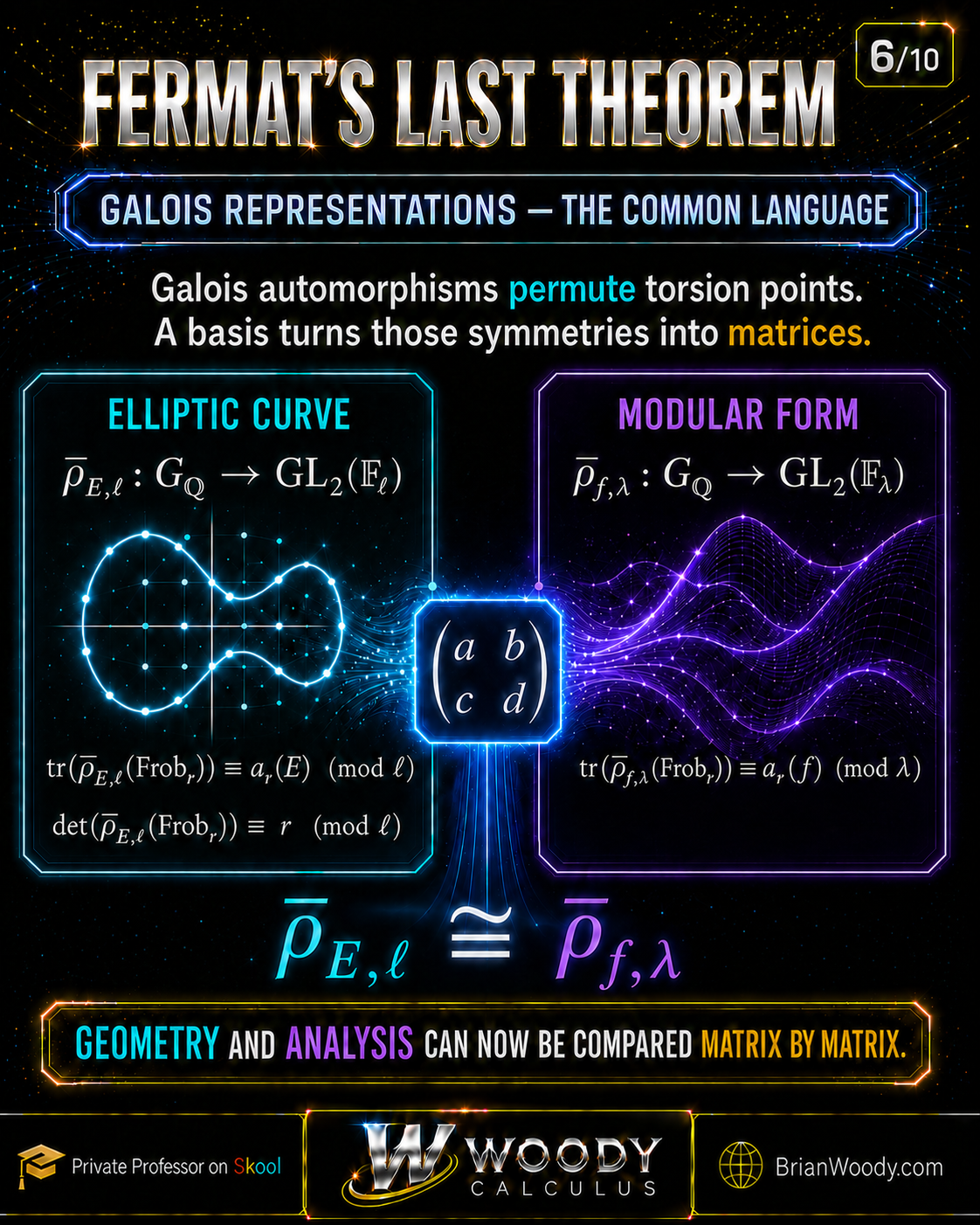
The elliptic-curve part attached arithmetic data to an elliptic curve by counting points modulo primes. The modular-form part found the same data inside the Fourier coefficients of a modular form:
a_r(E)=a_r(f).
\]
That numerical match tells us what modularity looks like. It does not yet explain why elliptic curves and modular forms can be compared deeply enough to prove it.
The missing bridge is a Galois representation.
Classical Galois Theory studies how field automorphisms permute the roots of polynomials. An elliptic curve contains torsion points whose coordinates are algebraic numbers. Galois automorphisms permute those points while respecting elliptic-curve addition.
Because the torsion points form a two-dimensional finite module, the permutation becomes a matrix:
\boxed{
\text{Galois symmetry}
\quad\longrightarrow\quad
\text{a }2\times2\text{ matrix.}
}
\]
Modular forms also produce two-dimensional Galois representations. Wiles’s proof operates on these linear representations, not by trying to compare the visible graph of a curve with the visible graph of a complex function.
Classical Galois Theory in One Precise Idea
Let
g(x)\in\mathbb Q[x]
\]
and let \(K\) be its splitting field over \(\mathbb Q\). The Galois group
\operatorname{Gal}(K/\mathbb Q)
\]
consists of field automorphisms of \(K\) that fix every rational number.
An automorphism must send a root of \(g\) to another root because
g(\alpha)=0
\quad\Longrightarrow\quad
g(\sigma(\alpha))
=\sigma(g(\alpha))
=0.
\]
Thus a Galois group acts by permuting roots while preserving every algebraic relation defined over \(\mathbb Q\).
For a cubic polynomial, the Galois group often sits inside
S_3,
\]
the group of permutations of its three roots.
Elliptic-curve Galois representations begin with this familiar action and add one crucial feature: the objects being permuted also form an abelian group.
Torsion Points on an Elliptic Curve
Let \(E/\mathbb Q\) be an elliptic curve. For a positive integer \(n\), define
E[n]
=\{P\in E(\overline{\mathbb Q}):nP=\mathcal O\}.
\]
These are the \(n\)-torsion points.
Over a field of characteristic zero,
E[n]\cong
(\mathbb Z/n\mathbb Z)^2.
\]
For a prime \(\ell\),
E[\ell]\cong\mathbb F_\ell^2.
\]
So \(E[\ell]\) is a two-dimensional vector space over the finite field \(\mathbb F_\ell\), containing
\ell^2
\]
points, including \(\mathcal O\).
For example,
E[2]\cong(\mathbb Z/2\mathbb Z)^2
\]
has four elements: the identity and three nonzero points of order \(2\).
Why torsion coordinates are algebraic
The condition
nP=\mathcal O
\]
can be expressed through polynomial equations in the coordinates of \(P\). Therefore torsion-point coordinates lie in finite algebraic extensions of \(\mathbb Q\).
That makes them natural objects for Galois Theory.
A Complete Example: The \(2\)-Torsion of Our Curve
Return to the curve used throughout the preceding elliptic-curve and modular-form discussion:
E:\quad y^2=x^3-x+1.
\]
A point \(P=(x,y)\) has order \(2\) exactly when
P=-P.
\]
Since
-(x,y)=(x,-y),
\]
this requires
y=0.
\]
The nonzero \(2\)-torsion points therefore have the form
(r_i,0),
\]
where \(r_1,r_2,r_3\) are the roots of
h(x)=x^3-x+1.
\]
Thus
E[2]
=\{\mathcal O,(r_1,0),(r_2,0),(r_3,0)\}.
\]
The splitting field of the cubic is exactly the field generated by the coordinates of the \(2\)-torsion points.
Step 1: prove the cubic is irreducible
The only possible rational roots are \(\pm1\). But
h(1)=1
\]
and
h(-1)=1.
\]
Therefore \(h(x)\) has no rational root. Since it is cubic, it is irreducible over \(\mathbb Q\).
Step 2: compute its discriminant
For
x^3+Ax+B,
\]
the polynomial discriminant is
\operatorname{disc}(h)=-4A^3-27B^2.
\]
Here \(A=-1\) and \(B=1\), so
\operatorname{disc}(h)
=-4(-1)^3-27(1)^2
=4-27
=-23.
\]
This is not a square in \(\mathbb Q\).
An irreducible cubic over \(\mathbb Q\) with nonsquare discriminant has Galois group
\operatorname{Gal}(h)\cong S_3.
\]
Step 3: identify the matrix group
Because
E[2]\cong\mathbb F_2^2,
\]
its invertible linear transformations form
\operatorname{GL}_2(\mathbb F_2).
\]
The order of this group is
|\operatorname{GL}_2(\mathbb F_2)|
=(2^2-1)(2^2-2)
=3\cdot2
=6.
\]
The group acts faithfully on the three nonzero vectors of \(\mathbb F_2^2\), so
\operatorname{GL}_2(\mathbb F_2)\cong S_3.
\]
Therefore the Galois action on \(E[2]\) is as large as possible:
\boxed{
\bar\rho_{E,2}:
G_{\mathbb Q}\twoheadrightarrow
\operatorname{GL}_2(\mathbb F_2)
\cong S_3.
}
\]
We have turned the classical Galois group of a cubic into the mod-\(2\) representation of an elliptic curve.
Constructing the Mod-\(\ell\) Representation
Let
G_{\mathbb Q}
=\operatorname{Gal}(\overline{\mathbb Q}/\mathbb Q)
\]
be the absolute Galois group of \(\mathbb Q\).
Because the equation of \(E\) has rational coefficients, every
\sigma\in G_{\mathbb Q}
\]
sends a torsion point to another torsion point. It also preserves addition:
\sigma(P+Q)=\sigma(P)+\sigma(Q).
\]
Thus \(\sigma\) acts linearly on the two-dimensional vector space \(E[\ell]\).
After choosing a basis of \(E[\ell]\), this action becomes a matrix, producing the continuous homomorphism
\boxed{
\bar\rho_{E,\ell}:
G_{\mathbb Q}
\longrightarrow
\operatorname{GL}_2(\mathbb F_\ell).
}
\]
This is the mod-\(\ell\) Galois representation attached to \(E\).
Does the representation depend on the basis?
The matrices do. The arithmetic representation does not.
Changing the basis conjugates every matrix by the same invertible matrix. Therefore the representation is naturally defined up to conjugacy.
Basis-independent quantities include:
- the trace,
- the determinant,
- the characteristic polynomial,
- reducibility or irreducibility,
- the image up to conjugacy.
These are precisely the invariants used throughout the proof of Fermat’s Last Theorem.
Frobenius: Recovering Point Counts from Matrices
Let \(r\) be a prime where \(E\) has good reduction, and assume
r\ne\ell.
\]
Then the mod-\(\ell\) representation is unramified at \(r\), so an arithmetic Frobenius element
\operatorname{Frob}_r
\]
has a well-defined conjugacy class in the representation.
The characteristic polynomial is
\boxed{
X^2-a_r(E)X+r
\pmod\ell,
}
\]
where
a_r(E)=r+1-\#E(\mathbb F_r).
\]
Consequently,
\operatorname{tr}\!\left(
\bar\rho_{E,\ell}(\operatorname{Frob}_r)
\right)
\equiv a_r(E)\pmod\ell
\]
and
\det\!\left(
\bar\rho_{E,\ell}(\operatorname{Frob}_r)
\right)
\equiv r\pmod\ell.
\]
The point-count coefficient from the modular-form part is now the trace of a Galois matrix.
This is the central translation:
\boxed{
r+1-\#E(\mathbb F_r)
=\text{Frobenius trace}.
}
\]
Frobenius in the Concrete Mod-\(2\) Example
Our curve has conductor
92=2^2\cdot23,
\]
so it has good reduction at \(3\) and \(5\).
Prime \(r=3\): a three-cycle
The modular-form part computed
a_3(E)=-3.
\]
Modulo \(2\),
a_3(E)\equiv1,
\qquad
3\equiv1.
\]
The Frobenius characteristic polynomial becomes
X^2+X+1
\]
over \(\mathbb F_2\). This is the characteristic polynomial of an order-three element of \(\operatorname{GL}_2(\mathbb F_2)\). Up to a choice of basis, one representative is
\begin{pmatrix}0&1\\1&1\end{pmatrix}.
\]
The same conclusion is visible from the cubic. Modulo \(3\),
x^3-x+1
\]
has no root, so it remains irreducible. Frobenius cyclically permutes its three roots—a three-cycle in \(S_3\).
The permutation description and the matrix-trace description agree.
Prime \(r=5\): a transposition
The modular-form part computed
a_5(E)=-2.
\]
Modulo \(2\),
a_5(E)\equiv0,
\qquad
5\equiv1,
\]
so the characteristic polynomial is
X^2+1=(X+1)^2.
\]
Meanwhile, the cubic factors modulo \(5\) as
x^3-x+1
=(x-3)(x^2+3x+3).
\]
The quadratic factor is irreducible modulo \(5\), so Frobenius fixes one root and exchanges the other two. It acts as a transposition.
Up to a choice of basis, a representative transposition matrix is
\begin{pmatrix}1&1\\0&1\end{pmatrix}.
\]
The characteristic polynomial alone does not distinguish every conjugacy possibility in characteristic \(2\), but the factorization pattern identifies the transposition.
These examples show that point counting, polynomial factorization, permutations of torsion points, and matrix traces are different views of the same Frobenius action.
The Determinant and the Weil Pairing
Why does the determinant of Frobenius equal \(r\pmod\ell\)?
The answer comes from the Weil pairing
e_\ell:
E[\ell]\times E[\ell]
\longrightarrow
\mu_\ell,
\]
where \(\mu_\ell\) is the group of \(\ell\)-th roots of unity.
The pairing is alternating, nondegenerate, and Galois equivariant:
e_\ell(\sigma P,\sigma Q)
=\sigma(e_\ell(P,Q)).
\]
The Galois action on roots of unity is recorded by the mod-\(\ell\) cyclotomic character
\bar\chi_\ell:
G_{\mathbb Q}
\longrightarrow
\mathbb F_\ell^\times.
\]
The Weil pairing forces
\det\bar\rho_{E,\ell}=\bar\chi_\ell.
\]
For arithmetic Frobenius at \(r\ne\ell\),
\bar\chi_\ell(\operatorname{Frob}_r)
\equiv r\pmod\ell.
\]
Therefore
\det\bar\rho_{E,\ell}(\operatorname{Frob}_r)
\equiv r\pmod\ell.
\]
The trace records the elliptic-curve point count. The determinant records the cyclotomic action.
Ramification and Bad Reduction
Galois representations also detect where an elliptic curve has bad reduction.
For a prime \(r\ne\ell\), the Néron–Ogg–Shafarevich criterion states:
\boxed{
E\text{ has good reduction at }r
\iff
T_\ell(E)\text{ is unramified at }r.
}
\]
Thus the local behavior of the Galois representation remembers the geometry of the reduced curve.
Our worked curve has bad reduction only at
2\quad\text{and}\quad23.
\]
Its \(\ell\)-adic representation is therefore unramified away from
2,23,\ell.
\]
The conductor measures the depth and type of this ramification. For the Frey curve, the Fermat equation imposes unusually controlled local behavior. Ribet’s theorem will exploit that control to lower the level of a modular representation.
From \(E[\ell]\) to the Tate Module
The mod-\(\ell\) representation sees only the \(\ell\)-torsion. To retain all powers of \(\ell\), consider
E[\ell],
E[\ell^2],
E[\ell^3],
\ldots
\]
linked by multiplication by \(\ell\).
The \(\ell\)-adic Tate module is the inverse limit
T_\ell(E)
=\varprojlim_n E[\ell^n].
\]
The inverse limit packages the compatible \(\ell^n\)-torsion data for every \(n\) into one object. Passing from the finite field \(\mathbb F_\ell\) to the \(\ell\)-adic integers \(\mathbb Z_\ell\), and then to \(\mathbb Q_\ell\), produces a characteristic-zero representation whose reduction modulo \(\ell\) recovers the residual representation. That characteristic-zero lift is the object needed in modularity-lifting arguments.
An element is a compatible sequence
(P_1,P_2,P_3,\ldots)
\]
with
P_n\in E[\ell^n]
\qquad\text{and}\qquad
\ell P_{n+1}=P_n.
\]
The Tate module is a free rank-two module over the \(\ell\)-adic integers:
T_\ell(E)\cong\mathbb Z_\ell^2.
\]
The Galois action produces the continuous \(\ell\)-adic representation
\boxed{
\rho_{E,\ell}:
G_{\mathbb Q}
\longrightarrow
\operatorname{GL}_2(\mathbb Z_\ell).
}
\]
Tensoring with \(\mathbb Q_\ell\) gives
V_\ell(E)
=T_\ell(E)\otimes_{\mathbb Z_\ell}\mathbb Q_\ell,
\]
a two-dimensional vector space over \(\mathbb Q_\ell\).
Reducing the \(\ell\)-adic representation modulo \(\ell\) recovers
\bar\rho_{E,\ell}.
\]
Residual Representations and Lifts
The mod-\(\ell\) representation
\bar\rho:
G_{\mathbb Q}\to\operatorname{GL}_2(\mathbb F_\ell)
\]
is called a residual representation.
A lift is a representation with coefficients in a larger \(\ell\)-adic ring that reduces to \(\bar\rho\) modulo its maximal ideal. Schematically,
\rho:
G_{\mathbb Q}\to\operatorname{GL}_2(A)
\]
is a lift when
\rho\pmod{\mathfrak m_A}=\bar\rho.
\]
Many lifts of the same residual representation may exist. Wiles imposes arithmetic conditions on the lifts:
- prescribed determinant,
- controlled ramification,
- specified behavior at \(\ell\),
- local conditions reflecting semistability.
Under the representability hypotheses used in Wiles’s setting—including the required irreducibility conditions—the collection of admissible lifts can be organized by a universal deformation ring
R.
\]
This is the first half of the eventual statement
R=\mathbf T.
\]
The other half, the Hecke algebra \(\mathbf T\), organizes lifts that come from modular forms.
Modular Forms Also Produce Galois Representations
Let
f(z)=\sum_{n=1}^{\infty}a_n(f)q^n
\]
be a normalized newform of weight \(k\), level \(N\), and character \(\chi\). Deligne’s theory attaches an \(\ell\)-adic Galois representation
\rho_{f,\lambda}:
G_{\mathbb Q}
\longrightarrow
\operatorname{GL}_2(K_{f,\lambda}),
\]
where \(K_{f,\lambda}\) is a completion of the coefficient field of \(f\) at a prime \(\lambda\) above \(\ell\).
For every prime \(r\nmid N\ell\),
\operatorname{tr}\rho_{f,\lambda}(\operatorname{Frob}_r)
=a_r(f)
\]
and
\det\rho_{f,\lambda}(\operatorname{Frob}_r)
=\chi(r)r^{k-1}.
\]
For the weight-two, trivial-character newforms attached to elliptic curves,
k=2,
\qquad
\chi=1,
\]
so the Frobenius characteristic polynomial is
X^2-a_r(f)X+r.
\]
Compare this with the elliptic-curve polynomial
X^2-a_r(E)X+r.
\]
If
a_r(E)=a_r(f)
\]
for every good prime, the characteristic polynomials match.
Why Matching Frobenius Data Determines the Representation
Frobenius elements are not a small or accidental subset of the Galois group. The Chebotarev Density Theorem says that their conjugacy classes are distributed densely enough to detect global Galois information.
Under the standard continuity and semisimplicity hypotheses, equality of Frobenius characteristic polynomials at almost all primes determines a representation up to semisimplification.
Thus modularity can be expressed as an isomorphism of compatible Galois representations:
\rho_{E,\ell}
\cong
\rho_{f,\lambda}
\]
in the appropriate sense.
This explains why the coefficient table from the modular-form part was so meaningful. Each equality
a_r(E)=a_r(f)
\]
was really a trace equality:
\operatorname{tr}\rho_{E,\ell}(\operatorname{Frob}_r)
=
\operatorname{tr}\rho_{f,\lambda}(\operatorname{Frob}_r).
\]
The arithmetic fingerprints match because the same Galois symmetry is being represented on both sides.
The Strategy of a Modularity-Lifting Theorem
Wiles’s central type of result can now be stated in conceptual form:
Begin with a residual representation \(\bar\rho\) already known to be modular. Prove that every sufficiently well-behaved \(\ell\)-adic lift of \(\bar\rho\) is also modular.
The logic is
\boxed{
\bar\rho\text{ is modular}
+\text{ local conditions on }\rho
\Longrightarrow
\rho\text{ is modular.}
}
\]
The residual representation is finite and therefore more accessible. The full \(\ell\)-adic representation contains the arithmetic of the elliptic curve. A modularity-lifting theorem transfers modularity from the finite approximation to the full object.
This is why the words residual, lift, and deformation are indispensable to Wiles’s proof.
The Frey Curve’s Representation
Suppose a primitive Fermat counterexample exists:
a^p+b^p=c^p,
\qquad
p\ge5\text{ prime}.
\]
Attach the Frey curve
E_{a,b,p}:
y^2=x(x-a^p)(x+b^p).
\]
The exponent prime \(p\) also supplies the mod-\(p\) representation
\bar\rho_{E_{a,b,p},p}:
G_{\mathbb Q}
\longrightarrow
\operatorname{GL}_2(\mathbb F_p).
\]
The special discriminant
\Delta=16(abc)^{2p}
\]
forces unusually controlled local behavior in this representation. Ribet’s level-lowering theorem uses that behavior to remove the primes dividing \(abc\) from the modular level.
Do not confuse two uses of primes in the full proof:
- In the Frey–Ribet step, the representation prime is naturally the Fermat exponent \(p\).
- In Wiles’s modularity-lifting argument for a general semistable elliptic curve, the primes \(3\) and \(5\) play special auxiliary roles.
The next part shows how the Frey representation is forced down to level \(2\), where the required modular form does not exist.
Part VI — Frey, Serre, and Ribet: Why the Hypothetical Curve Cannot Be Modular
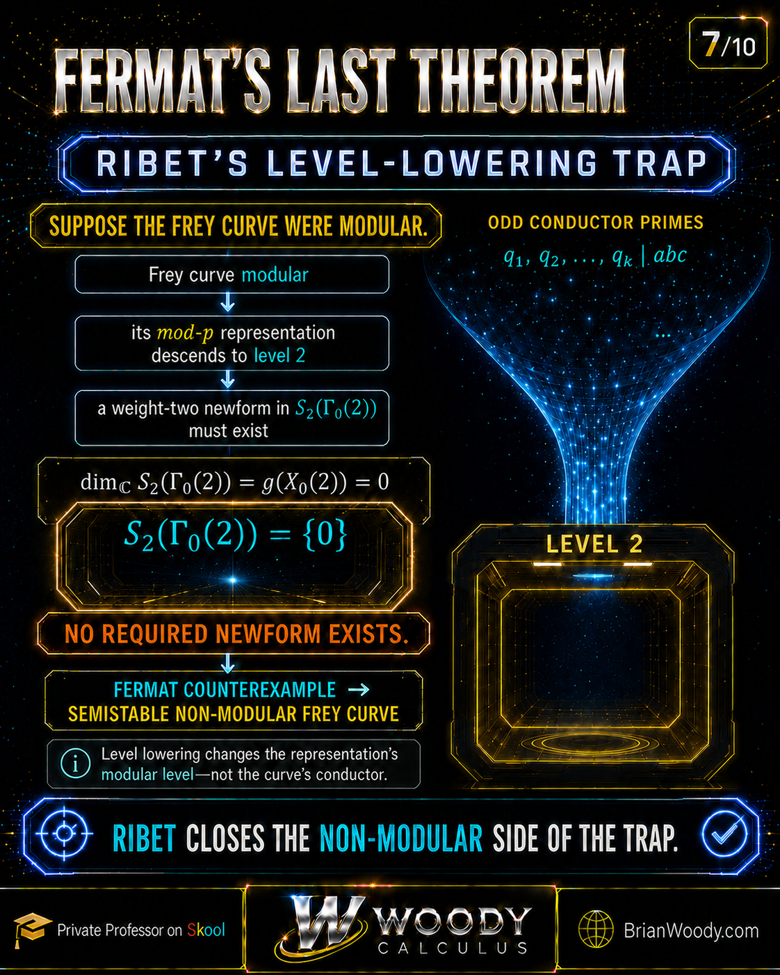
The Galois-representation part translated elliptic curves and modular forms into the same language: two-dimensional Galois representations.
Now that language springs the trap.
Assume, against Fermat’s Last Theorem, that there is a primitive solution
a^p+b^p=c^p,
\qquad
p\ge 5\text{ prime},
\qquad
\gcd(a,b,c)=1.
\]
From those three integers, construct the Frey curve
E_{a,b,p}:y^2=x(x-a^p)(x+b^p).
\]
Its discriminant contains enormous powers of the primes dividing \(abc\). That arithmetic peculiarity makes the curve semistable, yet makes its mod-\(p\) Galois representation behave as though most of those bad primes were absent.
Ribet’s level-lowering theorem turns that tension into an impossibility:
\boxed{
\text{If the Frey curve were modular, its mod-}p
\text{ representation would come from level }2.
}
\]
But there is no weight-two cusp form at level \(2\):
S_2(\Gamma_0(2))=\{0\}.
\]
Therefore the hypothetical Frey curve cannot be modular.
This does not yet prove Fermat’s Last Theorem. It completes one side of the final contradiction. Wiles will provide the other side by proving that every semistable elliptic curve over \(\mathbb Q\)—including any Frey curve—must be modular.
Begin with a Counterexample That Does Not Exist
A proof by contradiction temporarily grants its opponent everything it asks for.
Suppose
x^n+y^n=z^n
\]
has a nonzero integer solution for some \(n>2\).
As established in the exponent-reduction section, it is enough to consider prime exponents \(p\ge 5\). We may also divide out the common factor of \(x,y,z\), producing a primitive solution
a^p+b^p=c^p,
\qquad
\gcd(a,b,c)=1.
\]
Primitivity implies that \(a,b,c\) are pairwise coprime. If a prime divided two of them, the Fermat equation would force it to divide the third.
Exactly one of \(a,b,c\) is even. They cannot all be odd because
a^p+b^p\equiv 1+1\equiv 0\pmod 2
\]
would make \(c\) even, contradicting primitivity. Nor can two be even.
After interchanging \(a\) and \(b\) and making the standard sign choices, one can place the solution in a parity normalization convenient for the arithmetic at \(2\). The odd primes are comparatively transparent; the prime \(2\) is where the precise minimal model requires special care.
That warning will matter later. The slogan “remove every prime dividing \(abc\)” is almost right, but the rigorous conclusion is not level \(1\). The residual representation lands at level \(2\).
Attach the Frey Curve
To the hypothetical solution attach
E:y^2=x(x-a^p)(x+b^p).
\]
The right-hand side has roots
0,
\qquad
a^p,
\qquad
-b^p.
\]
They are distinct because \(abc\ne 0\), so this is an elliptic curve.
The curve has three visible nonzero points of order \(2\):
(0,0),
\qquad
(a^p,0),
\qquad
(-b^p,0).
\]
Thus
E[2](\mathbb Q)\cong
(\mathbb Z/2\mathbb Z)^2.
\]
The full rational \(2\)-torsion is not decorative. It is part of the unusually rigid arithmetic package created by a Fermat solution.
Compute the discriminant
For a curve
y^2=(x-r_1)(x-r_2)(x-r_3),
\]
the elliptic-curve discriminant of this displayed model is
16(r_1-r_2)^2(r_1-r_3)^2(r_2-r_3)^2.
\]
Here,
r_1-r_2=-a^p,
\qquad
r_1-r_3=b^p,
\]
and the Fermat equation gives
r_2-r_3=a^p+b^p=c^p.
\]
Therefore
\begin{aligned}
\Delta
&=16(a^p)^2(b^p)^2(c^p)^2\\
&=16(abc)^{2p}.
\end{aligned}
\]
So the hypothetical equation is encoded directly in the curve’s discriminant:
\boxed{\Delta=16(abc)^{2p}.}
\]
Every odd prime \(q\mid abc\) occurs in this discriminant to an exponent divisible by \(p\):
v_q(\Delta)=2p\,v_q(abc).
\]
This “too much divisibility by \(p\)” is exactly the feature that level lowering will exploit.
What the conductor remembers
The discriminant measures where the displayed cubic degenerates modulo a prime. The conductor measures the ramification and severity of bad reduction in a more economical way.
For the Frey curve:
- bad reduction is supported on primes dividing \(2abc\);
- after the standard normalization, the curve is semistable;
- at the relevant odd bad primes, the reduction is multiplicative;
- each such prime appears only once in the elliptic curve’s conductor.
The exact power of \(2\) in a minimal discriminant or conductor depends on the chosen integral model and parity normalization. That local calculation should not be replaced by casual cancellation.
The important contrast is this:
\begin{array}{c|c}
\text{Minimal discriminant} & \text{Conductor}\\
\hline
\text{remembers large valuations such as multiples of }p
& \text{records an odd multiplicative prime once}
\end{array}
\]
The residual Galois representation can forget even more than the curve’s conductor does.
Four Mathematicians Built the Bridge
The sentence “Ribet connected Fermat to modularity” compresses a remarkable chain of ideas. The proof is clearer—and the history fairer—when each link is visible.
Yves Hellegouarch: the arithmetic precursor
In work beginning in the 1960s, Yves Hellegouarch studied elliptic curves attached to putative Fermat solutions. The fundamental move of turning a Diophantine solution into an elliptic curve did not appear from nowhere in the 1980s.
Gerhard Frey: the audacious incompatibility
Gerhard Frey emphasized that a counterexample to Fermat would create an extraordinarily unusual semistable elliptic curve. Its discriminant and conductor seemed incompatible with what modularity should permit.
Frey’s insight was not merely “associate a curve.” It was:
\boxed{
\text{A Fermat counterexample should manufacture a curve too strange to be modular.}
}
\]
That was a daring bridge between a seventeenth-century equation and the modern arithmetic of modular curves.
But a compelling incompatibility is not yet a theorem. The exact obstruction had to be formulated.
Jean-Pierre Serre: the precise prediction
Jean-Pierre Serre translated Frey’s idea into the language of mod-\(p\) Galois representations. His epsilon conjecture predicted the missing level-lowering step.
The point was not that the Frey curve’s own conductor literally becomes \(2\). Rather, if the curve were modular, the residual representation
\bar\rho_{E,p}:G_{\mathbb Q}
\longrightarrow
\operatorname{GL}_2(\mathbb F_p)
\]
would have to arise from a modular form of dramatically lower level.
For the normalized Frey curve, the predicted level was \(2\).
Kenneth Ribet: the theorem that closes the exit
Kenneth Ribet proved the required level-lowering result in 1986. His work established the bridge Frey and Serre had envisioned:
\boxed{
\text{Semistable modularity}
\quad\Longrightarrow\quad
\text{FLT}.
}
\]
Ribet did not prove semistable modularity. He proved that if mathematicians could establish it, no Fermat counterexample could survive.
That transformed Fermat’s Last Theorem. Instead of attacking infinitely many equations directly, one could attack a precise modularity problem for semistable elliptic curves over \(\mathbb Q\).
What “The Frey Curve Is Modular” Would Mean
Suppose, temporarily, that the Frey curve \(E\) were modular.
Let \(N_E\) be its conductor. Modularity would supply a normalized weight-two newform
f(q)=\sum_{n=1}^{\infty}a_n(f)q^n
\in S_2(\Gamma_0(N_E))
\]
whose \(L\)-function matches that of \(E\).
For every prime \(r\nmid N_E\),
a_r(f)=a_r(E)
=r+1-\#E(\mathbb F_r).
\]
The Galois-representation part expressed the same equality through Galois representations. Reducing modulo the Fermat exponent \(p\), the modular form and curve would give isomorphic residual representations:
\bar\rho_{f,p}
\cong
\bar\rho_{E,p}.
\]
Equivalently, away from the bad and representation primes,
a_r(f)\equiv a_r(E)\pmod p.
\]
The representation \(\bar\rho_{E,p}\), rather than the original equation or even the curve by itself, is the object Ribet lowers.
Level Lowering Does Not Change the Curve
This distinction is one of the most important in the entire proof.
The incorrect picture
It is incorrect to imagine that Ribet repeatedly edits the Frey curve until its conductor becomes \(2\):
E\rightsquigarrow E^{\prime}\rightsquigarrow
\text{an elliptic curve of conductor }2.
\]
No such conductor-\(2\) elliptic curve is being constructed.
The correct picture
The Frey curve remains the same curve. Its conductor remains its conductor. What changes is the level at which its mod-\(p\) representation would have to occur.
Schematically, if a newform \(f\) of level \(N\) gives a residual representation
\bar\rho,
\]
and Ribet’s hypotheses hold at a prime \(q\mid N\), level lowering produces a newform \(g\) of lower level \(M\mid N\) with
\bar\rho_{g,p}\cong\bar\rho_{f,p}.
\]
For almost all primes \(r\), this means
a_r(g)\equiv a_r(f)\pmod p.
\]
The integral coefficients need not be equal. Their reductions encode the same mod-\(p\) representation.
The operation is therefore
\boxed{
\text{same residual representation, lower modular level.}
}
\]
It is not
\boxed{
\text{same curve, lower curve conductor.}
}
\]
Why the Odd Primes Can Disappear
Consider an odd prime \(q\mid abc\) with \(q\ne p\). At such a prime, the Frey curve has multiplicative reduction, so \(q\) contributes to the conductor of the curve.
Yet
v_q(\Delta)=2p\,v_q(abc)
\]
is divisible by \(p\).
For a multiplicative prime, the local Galois action on the \(p\)-torsion is governed by a unipotent extension. When the relevant discriminant valuation is divisible by \(p\), the mod-\(p\) representation loses the ramification that the full curve still remembers.
In a simplified local slogan:
\begin{array}{c}
q\mid N_E
\quad\text{because the curve has bad reduction},\\[4pt]
\text{but }q\nmid N(\bar\rho_{E,p})
\quad\text{because the mod-}p\text{ representation is unramified there.}
\end{array}
\]
That is why a prime can appear in the conductor of the curve but disappear from the conductor—or Serre level—of its residual representation.
Ribet’s theorem turns this local disappearance into a global modular statement: if the representation came from a modular form at the original level, it must also come from a modular form with that prime removed from the level.
Why this explanation needs a qualification at \(p\)
The prime used in the representation is itself \(p\), the Fermat exponent. Local behavior at that prime is subtler than the case \(q\ne p\). Likewise, the prime \(2\) requires a dedicated minimal-model analysis.
The rigorous Frey–Serre–Ribet argument handles these places through the precise local conditions and parity normalization. The safe conclusion is:
\boxed{
N(\bar\rho_{E,p})=2
}
\]
for the relevant irreducible odd representation attached to the normalized Frey curve.
The valuation calculation explains the mechanism at the ordinary odd bad primes. It should not be mistaken for a complete proof of every local case by itself.
The Descent to Level 2
Now combine modularity with level lowering.
Assume the Frey curve is modular. Then its mod-\(p\) representation comes from a weight-two newform at the curve’s conductor.
Ribet’s theorem removes the removable odd primes contributed by \(abc\). The special local analysis at \(2\) leaves level \(2\).
Therefore there would have to exist a normalized cusp eigenform
g\in S_2(\Gamma_0(2))
\]
such that
\bar\rho_{g,p}\cong\bar\rho_{E,p}.
\]
This is the precise pressure point:
\boxed{
\text{Frey curve modular}
\Longrightarrow
\text{a weight-two newform of level }2.
}
\]
The proof does not now wave toward a mysterious classification table. We can calculate the relevant space directly.
Why No Weight-Two Cusp Form Exists at Level 2
Weight-two cusp forms have a geometric interpretation. If
f(z)\in S_2(\Gamma_0(N)),
\]
then
f(z)\,dz
\]
descends to a holomorphic differential on the compact modular curve \(X_0(N)\). Conversely, every holomorphic differential on \(X_0(N)\) arises this way.
Therefore
\dim_{\mathbb C}S_2(\Gamma_0(N))
=g(X_0(N)),
\]
where \(g(X_0(N))\) is the genus of the modular curve.
So we only need the genus of \(X_0(2)\).
Step 1: compute the index
The index of \(\Gamma_0(N)\) in \(\operatorname{SL}_2(\mathbb Z)\) is
\mu(N)
=N\prod_{q\mid N}\left(1+\frac1q\right).
\]
For \(N=2\),
\mu(2)
=2\left(1+\frac12\right)
=3.
\]
Step 2: count the special points
For \(\Gamma_0(2)\):
- the number of cusps is \(c=2\);
- the number of elliptic fixed-point orbits of order \(2\) is \(e_2=1\);
- the number of elliptic fixed-point orbits of order \(3\) is \(e_3=0\).
Geometrically, the two cusps may be represented by
\infty
\qquad\text{and}\qquad
0.
\]
Step 3: use the genus formula
The genus formula is
g(X_0(N))
=1+\frac{\mu}{12}
-\frac{e_2}{4}
-\frac{e_3}{3}
-\frac{c}{2}.
\]
Substituting the level-\(2\) data,
\begin{aligned}
g(X_0(2))
&=1+\frac{3}{12}
-\frac14
-0
-\frac22\\
&=1+\frac14-\frac14-1\\
&=0.
\end{aligned}
\]
Consequently,
\dim_{\mathbb C}S_2(\Gamma_0(2))=0.
\]
Hence
\boxed{S_2(\Gamma_0(2))=\{0\}.}
\]
There is no nonzero weight-two cusp form at level \(2\), and therefore no normalized weight-two newform at level \(2\).
A subtle but important wording choice
The conclusion is not “there are no modular forms of any kind at level \(2\).” Eisenstein and noncuspidal phenomena are a different matter.
The Frey representation would require a weight-two cuspidal eigenform. That is the space that vanishes.
The Non-Modularity Contradiction
We can now place the argument on one page.
Assume a primitive Fermat counterexample exists:
a^p+b^p=c^p,
\qquad p\ge5.
\]
Attach the Frey curve
E:y^2=x(x-a^p)(x+b^p).
\]
It is a semistable elliptic curve over \(\mathbb Q\).
Now suppose \(E\) is modular. Its mod-\(p\) representation must arise from a weight-two newform.
Ribet’s level-lowering theorem forces that representation to arise at level \(2\):
g\in S_2(\Gamma_0(2)).
\]
But
S_2(\Gamma_0(2))=\{0\}.
\]
No such \(g\) exists. Therefore the assumption that \(E\) is modular is impossible.
Thus
\boxed{
\text{Fermat counterexample}
\Longrightarrow
\text{a semistable non-modular elliptic curve.}
}
\]
This is the Frey–Serre–Ribet half of the proof.
What Ribet Proved—and What He Did Not
Ribet’s theorem is sometimes summarized so aggressively that the logic becomes historically and mathematically wrong.
Ribet did prove
Ribet proved the needed level-lowering result and thereby established that semistable modularity would imply Fermat’s Last Theorem.
In implication form:
\boxed{
\left(
\begin{array}{c}
\text{every semistable elliptic curve}\\
\text{over }\mathbb Q\text{ is modular}
\end{array}
\right)
\Longrightarrow
\text{FLT}.
}
\]
Ribet did not prove
He did not prove that every semistable elliptic curve is modular. That was the immense remaining problem.
Wiles would prove
Wiles, with the repaired argument completed alongside Richard Taylor, proved the semistable case needed here:
\boxed{
\text{Every semistable elliptic curve over }\mathbb Q
\text{ is modular.}
}
\]
The two conclusions collide:
\begin{array}{rcl}
\text{Fermat counterexample}
&\Longrightarrow&
\text{semistable Frey curve},\\[4pt]
\text{Ribet}
&\Longrightarrow&
\text{Frey curve is not modular},\\[4pt]
\text{Wiles–Taylor}
&\Longrightarrow&
\text{Frey curve is modular}.
\end{array}
\]
A curve cannot be both modular and non-modular. Therefore the opening counterexample cannot exist.
The Entire Logical Spine of Fermat’s Last Theorem
At this point the proof’s global architecture can be seen without hiding any bridge behind a slogan.
The hypothetical arithmetic object
a^p+b^p=c^p
\]
creates
E:y^2=x(x-a^p)(x+b^p).
\]
The elliptic curve creates a representation
\bar\rho_{E,p}:G_{\mathbb Q}
\to\operatorname{GL}_2(\mathbb F_p).
\]
Ribet controls the modular level
If \(E\) were modular, then
\bar\rho_{E,p}
\]
would arise from a weight-two newform at level \(2\).
Geometry closes that destination
g(X_0(2))=0
\Longrightarrow
S_2(\Gamma_0(2))=0.
\]
So the Frey curve cannot be modular.
Wiles closes the other exit
The Frey curve is semistable, and Wiles proves every semistable elliptic curve over \(\mathbb Q\) is modular.
Therefore
\boxed{
\text{No Fermat counterexample exists.}
}
\]
The last line is short because centuries of mathematics have been compressed into the arrows above it.
Why Level 2 Is Such a Devastating Destination
Level lowering is powerful because small levels contain very little room.
The original Frey curve can have a large conductor involving many primes dividing \(abc\). At a large level, one might reasonably expect many modular forms.
But the residual representation forgets those removable primes. Its predicted level collapses to \(2\), where the associated modular curve has genus zero.
A genus-zero compact Riemann surface has no nonzero holomorphic differentials. Since weight-two cusp forms are precisely those differentials,
\text{genus zero}
\Longrightarrow
\text{no weight-two cusp forms}.
\]
This is more than a low-level lookup. It is a geometric impossibility.
The counterexample begins by seeming to create an exotic elliptic curve. Ribet forces the essential representation of that curve into a modular space too small to contain it.
Serre’s Epsilon Conjecture and Serre’s Broader Vision
Two related ideas should not be collapsed into one.
The epsilon conjecture was the specific level-lowering prediction needed for the Frey curve argument. Ribet proved the relevant theorem.
Serre also formulated a much broader conjecture describing which odd, irreducible, two-dimensional mod-\(p\) Galois representations arise from modular forms and predicting their weights and levels.
That broader modularity conjecture reached far beyond Fermat’s Last Theorem. It was proved much later through work of Chandrashekhar Khare and Jean-Pierre Wintenberger, with an important refinement by Mark Kisin.
For the logic of Fermat’s Last Theorem, however, the indispensable 1986 breakthrough was Ribet’s level lowering for the Frey representation.
Part VII — Wiles’s Strategy: From One Modular Shadow to Every Admissible Lift
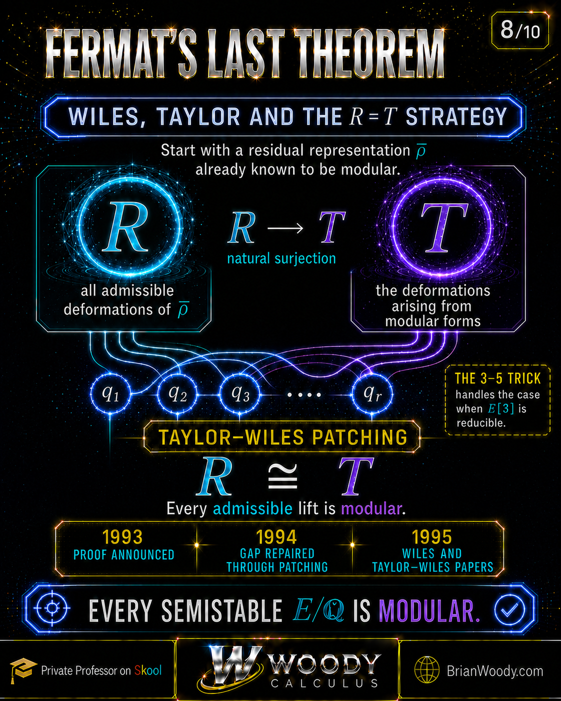
The preceding Frey–Serre–Ribet part completed the Frey–Serre–Ribet half of the proof:
\boxed{
\text{Fermat counterexample}
\Longrightarrow
\text{a semistable elliptic curve that cannot be modular.}
}
\]
The remaining task sounds simple:
\boxed{
\text{Prove every semistable elliptic curve over }\mathbb Q
\text{ is modular.}
}
\]
It was anything but simple.
Wiles did not construct a modular form directly from each elliptic curve. He changed the question. Instead of comparing curves with modular forms all at once, he compared their Galois representations one layer at a time.
Fix a prime \(p\). An elliptic curve \(E/\mathbb Q\) gives a residual representation
\bar\rho_{E,p}:G_{\mathbb Q}
\longrightarrow
\operatorname{GL}_2(\mathbb F_p)
\]
and a full \(p\)-adic representation
\rho_{E,p}:G_{\mathbb Q}
\longrightarrow
\operatorname{GL}_2(\mathbb Z_p).
\]
The second reduces to the first modulo \(p\):
\rho_{E,p}\pmod p
=\bar\rho_{E,p}.
\]
Wiles’s strategy was to begin with a residual representation already known to be modular and then prove that every lift satisfying the correct arithmetic conditions is modular too.
In its most memorable form:
\boxed{
\text{modular residual seed}
+
\text{controlled lift}
\Longrightarrow
\text{modular lift}.
}
\]
The machine that makes that implication possible is the comparison
\boxed{R\cong\mathbf T.}
\]
The deformation ring \(R\) describes all admissible Galois lifts. The Hecke algebra \(\mathbf T\) describes the lifts known to come from modular forms. If the rings are identical, there is no room for a permitted non-modular lift to hide.
Wiles Attacked the Representation, Not the Fermat Equation
After Ribet’s theorem, Wiles did not need to manipulate
a^p+b^p=c^p
\]
directly. Nor did he need to prove the full modularity conjecture for every elliptic curve over \(\mathbb Q\).
He needed the semistable case.
A semistable elliptic curve has only good or multiplicative reduction at every prime. Its conductor is squarefree. The hypothetical Frey curve belongs to this class.
Therefore the decisive theorem was:
\boxed{
E/\mathbb Q\text{ semistable}
\Longrightarrow
E\text{ modular}.
}
\]
Suppose \(E\) is an arbitrary semistable elliptic curve. To prove \(E\) modular, it is enough to prove that one of its \(p\)-adic Galois representations is modular. That is, we seek a modular eigenform \(f\) and a prime \(\lambda\mid p\) such that
\rho_{E,p}
\cong
\rho_{f,\lambda},
\]
with the appropriate identification of coefficient fields.
At almost every prime \(q\), this is reflected in the equality
\operatorname{tr}\rho_{E,p}(\operatorname{Frob}_q)
=a_q(E)
=a_q(f).
\]
The problem is still enormous: a \(p\)-adic representation contains infinitely much compatible information modulo
p,
\quad p^2,
\quad p^3,
\quad\ldots.
\]
Wiles’s first conceptual victory was recognizing that the mod-\(p\) layer could serve as a foothold.
Residual Modularity Is the Seed
Let \(\mathcal O\) be the ring of integers in a finite extension of \(\mathbb Q_p\), with maximal ideal \(\mathfrak m\) and residue field
k=\mathcal O/\mathfrak m.
\]
Suppose
\bar\rho:G_{\mathbb Q}
\longrightarrow
\operatorname{GL}_2(k)
\]
is continuous, odd, and irreducible.
The representation is odd when complex conjugation \(c\in G_{\mathbb Q}\) satisfies
\det\bar\rho(c)=-1.
\]
It is modular if there is a modular eigenform \(f\) and a prime \(\lambda\mid p\) in its coefficient field such that
\bar\rho
\cong
\bar\rho_{f,\lambda}.
\]
This does not yet say that a particular \(p\)-adic lift \(\rho\) of \(\bar\rho\) is modular. Many different \(p\)-adic representations can reduce to the same residual representation.
The logic Wiles needed was therefore not
\bar\rho\text{ modular}
\Longrightarrow
\text{every imaginable lift is modular}.
\]
That statement is far too broad.
He needed a theorem of the form
\boxed{
\begin{array}{c}
\bar\rho\text{ modular and sufficiently irreducible},\\
\rho\text{ satisfies specified local and global conditions}
\end{array}
\Longrightarrow
\rho\text{ modular}.
}
\]
This is a modularity-lifting theorem.
It moves upward from a modular mod-\(p\) representation to a modular \(p\)-adic representation. Ribet’s theorem moved downward in modular level. The two processes have different inputs, different outputs, and different roles.
Why the Prime 3 Opens the Door
Why not begin with an arbitrary prime?
The prime \(3\) has an exceptional advantage. The group
\operatorname{PGL}_2(\mathbb F_3)
\cong S_4
\]
is solvable. Consequently, the finite projective image of an irreducible mod-\(3\) representation lies in a class reached by the work of Robert Langlands and Jerrold Tunnell.
The Langlands–Tunnell theorem
In the form Wiles uses, Langlands–Tunnell begins with a continuous, irreducible, odd, two-dimensional complex Galois representation with finite solvable image and produces a weight-one newform with the same Artin \(L\)-function, up to the specified local factors.
For an elliptic curve \(E/\mathbb Q\), an irreducible representation
\bar\rho_{E,3}:G_{\mathbb Q}
\to\operatorname{GL}_2(\mathbb F_3)
\]
can be connected to such a finite-image complex representation. Langlands–Tunnell then supplies modularity.
But there is a detail that popular accounts often erase:
\boxed{
\text{Langlands–Tunnell naturally produces a weight-one form,}
\text{ not the final weight-two form.}
}
\]
Wiles multiplies the weight-one form by a suitable weight-one Eisenstein series congruent to \(1\) modulo \(3\). The product has weight \(2\) while retaining the required mod-\(3\) Hecke eigenvalues. A Deligne–Serre lifting argument then yields a weight-two eigenform with the same residual Galois representation.
Thus, under the necessary irreducibility hypotheses,
\boxed{
\bar\rho_{E,3}\text{ irreducible}
\Longrightarrow
\bar\rho_{E,3}\text{ modular}.
}
\]
This is the seed. It does not yet prove that the full representation
\rho_{E,3}:G_{\mathbb Q}\to\operatorname{GL}_2(\mathbb Z_3)
\]
is modular. That is the lifting problem Wiles had to solve.
What Is a Deformation?
Fix an irreducible residual representation
\bar\rho:G_{\mathbb Q}\to\operatorname{GL}_2(k).
\]
Let \(A\) be a complete local Noetherian \(\mathcal O\)-algebra with maximal ideal \(\mathfrak m_A\) and residue field \(k\).
A lift of \(\bar\rho\) to \(A\) is a continuous representation
\rho_A:G_{\mathbb Q}\to\operatorname{GL}_2(A)
\]
such that
\rho_A\pmod{\mathfrak m_A}
=\bar\rho.
\]
Two lifts are treated as the same deformation when they are conjugate by a matrix congruent to the identity modulo \(\mathfrak m_A\). This removes changes of basis that do not change the underlying arithmetic representation.
The coefficient ring \(A\) may be
k[\varepsilon]/(\varepsilon^2),
\qquad
\mathcal O/p^n\mathcal O,
\qquad
\mathcal O,
\]
or another suitable local ring.
Changing \(A\) lets us examine infinitesimal, finite-level, and full \(p\)-adic lifts within a single framework.
Not Every Lift Is Allowed
If we permit arbitrary ramification and arbitrary local behavior, the deformation problem becomes too large and the intended modularity statement becomes false or unmanageable.
Wiles imposes conditions modeled simultaneously on:
- the Galois representations coming from semistable elliptic curves;
- the Galois representations coming from modular forms.
The precise conditions depend on the case, but they control features such as:
- The determinant. For an elliptic curve, the determinant is the \(p\)-adic cyclotomic character: \[
\det\rho_{E,p}=\chi_p.
\] - Ramification outside a finite set. The lift may ramify only at designated primes.
- Minimal ramification. At many primes, the lift is required to introduce no more ramification than the residual representation already possesses.
- Behavior at \(p\). Wiles separates ordinary and finite-flat cases, capturing the local possibilities needed for semistable curves.
- Oddness and irreducibility. These are essential global constraints in the two-dimensional setting.
The phrase admissible deformation means a deformation satisfying the chosen package of local and global conditions.
This package is not technical clutter. It defines the exact universe in which a universal ring can be compared with a modular Hecke algebra.
The Universal Deformation Ring \(R\)
For each allowed coefficient ring \(A\), let
\mathcal D(A)
\]
denote the set of admissible deformations of \(\bar\rho\) to \(A\).
Under the required irreducibility hypotheses, Mazur’s deformation theory shows that this functor is represented by a complete local ring \(R\). That means there is a universal deformation
\rho^{\mathrm{univ}}:
G_{\mathbb Q}\to\operatorname{GL}_2(R)
\]
with the property that every admissible deformation \(\rho_A\) comes from a unique local \(\mathcal O\)-algebra homomorphism
\varphi:R\to A.
\]
The representation \(\rho_A\) is obtained by applying \(\varphi\) to the matrix entries of \(\rho^{\mathrm{univ}}\):
\rho_A
=
\varphi\circ\rho^{\mathrm{univ}}.
\]
Equivalently,
\boxed{
\operatorname{Hom}_{\mathcal O}^{\mathrm{local}}(R,A)
\cong
\mathcal D(A).
}
\]
Why “universal” is the right word
The ring \(R\) is not one chosen lift. It is the algebraic parameter space for all admissible lifts of \(\bar\rho\).
Its shape may be imagined schematically as
R\cong
\mathcal O[[X_1,\ldots,X_r]]
/(F_1,\ldots,F_s),
\]
where the variables represent deformation directions and the relations impose arithmetic constraints.
This display is a model of the structure, not a claim that Wiles’s rings always arrive with those particular variables or relations written explicitly.
Infinitesimal directions and Galois cohomology
The first-order deformations are obtained by taking
A=k[\varepsilon]/(\varepsilon^2).
\]
Their space is controlled by a Selmer group inside
H^1\!\left(G_{\mathbb Q},
\operatorname{ad}^0\bar\rho\right),
\]
where \(\operatorname{ad}^0\bar\rho\) is the three-dimensional space of trace-zero \(2\times2\) matrices, with Galois acting by conjugation.
This Selmer group is not the usual elliptic-curve Selmer group from the Birch and Swinnerton-Dyer conjecture. It is a deformation-theoretic Selmer group defined by the local conditions of the lifting problem.
In a compressed dictionary:
\begin{array}{c|c}
\text{Deformation theory} & \text{Galois cohomology}\\
\hline
\text{first-order deformation directions}
& H^1\text{ with local conditions}\\
\text{obstructions to extending a deformation}
& H^2\text{-type obstruction classes}
\end{array}
\]
This converts the size and complexity of \(R\) into cohomological questions that can be estimated.
The Hecke Algebra \(\mathbf T\)
Now approach the same residual representation from the modular side.
At the appropriate weight and level, Hecke operators
T_q,
\qquad U_q,
\qquad \langle d\rangle
\]
act on a space of modular forms. The algebra generated by these operators is a Hecke algebra.
The residual representation \(\bar\rho\) determines a maximal ideal \(\mathfrak m\) of this Hecke algebra through congruences such as
T_q
\equiv
\operatorname{tr}\bar\rho(\operatorname{Frob}_q)
\pmod{\mathfrak m}
\]
at the unramified primes.
Localizing and completing at \(\mathfrak m\) isolates the modular forms congruent to the residual seed. Denote the resulting local Hecke algebra by
\mathbf T.
\]
There is a Galois representation with coefficients in \(\mathbf T\):
\rho^{\mathrm{mod}}:
G_{\mathbb Q}\to\operatorname{GL}_2(\mathbf T)
\]
whose Frobenius traces satisfy
\operatorname{tr}\rho^{\mathrm{mod}}(\operatorname{Frob}_q)
=T_q
\]
away from the relevant bad primes.
Every characteristic-zero eigenform represented in this localized Hecke algebra gives a specialization
\mathbf T\to\mathcal O^{\prime}
\]
and therefore a modular \(p\)-adic Galois representation.
Thus
\boxed{
\mathbf T
=
\text{the algebraic parameter space for the modular lifts under consideration.}
}
\]
Why There Is a Natural Map \(R\to\mathbf T\)
The representation \(\rho^{\mathrm{mod}}\) is itself an admissible deformation of \(\bar\rho\). By the universal property of \(R\), it must arise from a homomorphism
\Phi:R\longrightarrow\mathbf T.
\]
Because the Hecke algebra is generated by the Frobenius data recorded by the universal representation, the map is surjective in the deformation problems Wiles constructs:
\boxed{R\twoheadrightarrow\mathbf T.}
\]
This direction is important.
The ring \(R\) describes every admissible lift. The ring \(\mathbf T\) describes those admissible lifts that are already known to be modular. Therefore the modular world is initially a quotient of the full deformation world.
There could, in principle, be a nonzero kernel:
\ker\Phi\ne0.
\]
Such a kernel would represent deformation information not detected by modular forms—the possible hiding place for non-modular lifts.
Wiles’s target was to prove that this hiding place is empty.
Why \(R=\mathbf T\) Proves Modularity Lifting
Suppose
\Phi:R\to\mathbf T
\]
is an isomorphism.
Let
\rho:G_{\mathbb Q}\to\operatorname{GL}_2(\mathcal O^{\prime})
\]
be any admissible \(p\)-adic lift of \(\bar\rho\). Universality produces a homomorphism
R\to\mathcal O^{\prime}.
\]
But if
R\cong\mathbf T,
\]
this homomorphism is simultaneously a Hecke-algebra specialization:
\mathbf T\to\mathcal O^{\prime}.
\]
Therefore the lift is represented by modular Hecke eigenvalues. It is modular.
The logical force is:
\begin{aligned}
R&=\text{all admissible lifts},\\
\mathbf T&=\text{modular admissible lifts},\\
R\cong\mathbf T
&\Longrightarrow
\text{all admissible lifts are modular}.
\end{aligned}
\]
Or, in one line:
\boxed{
R=\mathbf T
\Longrightarrow
\text{modularity lifts from }\bar\rho\text{ to }\rho.
}
\]
This is the structural heart of Wiles’s strategy.
What the equation does not mean
The symbols \(R\) and \(\mathbf T\) do not name two universal rings used identically in every theorem. The rings depend on:
- the residual representation;
- the determinant;
- the allowed ramification;
- the local condition at \(p\);
- the chosen modular weight and level.
There are minimal and nonminimal deformation problems, ordinary and finite-flat cases, and corresponding Hecke algebras.
So “Wiles proved \(R=\mathbf T\)” is a powerful summary, not a substitute for specifying which \(R\) and which \(\mathbf T\).
How Can Two Enormous Rings Be Proven Equal?
A surjection
R\twoheadrightarrow\mathbf T
\]
does not become an isomorphism through wishful thinking. One must prove the kernel vanishes.
Wiles compares infinitesimal information on both sides.
On the deformation side, the cotangent space of \(R\) is controlled by the deformation-theoretic Selmer group. On the Hecke side, congruence modules measure how modular forms with related systems of eigenvalues meet modulo powers of \(p\).
Very roughly, the comparison has the form
\boxed{
\text{size of permitted Galois deformations}
\quad\text{versus}\quad
\text{size of modular congruences}.
}
\]
If the Hecke algebra has the right complete-intersection structure and the two numerical measurements agree, a commutative-algebra criterion forces
R\cong\mathbf T.
\]
A local ring is a complete intersection when it can be presented as a quotient of a regular local ring by a regular sequence. In the finite-flat situations relevant here, this says the relations are as independent and as numerous as the expected dimension count demands.
The difficulty is that the required Selmer-group bounds and complete-intersection properties are themselves extremely deep. Establishing them is where auxiliary primes, patching, and the eventual Taylor–Wiles repair enter.
That is the next part.
For now, the architecture is complete:
\boxed{
\bar\rho\text{ modular}
\longrightarrow
R\twoheadrightarrow\mathbf T
\longrightarrow
R\cong\mathbf T
\longrightarrow
\rho\text{ modular}.
}
\]
The Easy Case: \(E[3]\) Is Irreducible
Let \(E/\mathbb Q\) be semistable and suppose
\bar\rho_{E,3}
\]
is irreducible.
Wiles verifies the stronger irreducibility and local hypotheses required by his lifting theorem. Semistability controls the ramification, including the ordinary or finite-flat behavior at \(3\).
The argument then runs as follows.
Step 1: obtain residual modularity
Langlands–Tunnell, together with the weight-raising and lifting step, gives
\bar\rho_{E,3}\text{ modular}.
\]
Step 2: recognize the full representation as an admissible lift
The \(3\)-adic Tate-module representation
\rho_{E,3}:G_{\mathbb Q}\to\operatorname{GL}_2(\mathbb Z_3)
\]
reduces to \(\bar\rho_{E,3}\) and satisfies the needed semistable local conditions.
Step 3: apply modularity lifting
The appropriate \(R=\mathbf T\) theorem forces
\rho_{E,3}\text{ modular}.
\]
Step 4: return to the elliptic curve
The modularity of the \(3\)-adic representation identifies the Frobenius traces of \(E\) with those of a weight-two newform. The isogeny theory of Faltings and Serre supplies the corresponding geometric modularity statement.
Therefore
\boxed{
E[3]\text{ irreducible}
\Longrightarrow
E\text{ modular}.
}
\]
This proves semistable modularity for a vast class of curves. One obstruction remains:
\bar\rho_{E,3}\text{ might be reducible}.
\]
Wiles’s deformation theory requires an irreducible residual representation. He needed a different modular seed.
The 3–5 Trick
Suppose \(E/\mathbb Q\) is semistable but
\bar\rho_{E,3}
\]
is reducible.
The Langlands–Tunnell route can no longer provide the irreducible seed required by Wiles’s lifting theorem.
The astonishing solution is not to force the mod-\(3\) representation to become irreducible. It is to move to the \(5\)-torsion, construct another elliptic curve, and then bring modularity back.
First exclude simultaneous reducibility
If both
\bar\rho_{E,3}
\qquad\text{and}\qquad
\bar\rho_{E,5}
\]
are reducible, \(E\) determines a rational point on the modular curve \(X_0(15)\), encoding compatible rational cyclic subgroups of orders \(3\) and \(5\).
Wiles uses the known rational points on \(X_0(15)\): the exceptional noncuspidal possibilities correspond to nonsemistable curves or to cases already known to be modular. Thus, for the unresolved semistable case, one may take
\bar\rho_{E,5}\text{ irreducible}.
\]
Construct a companion curve
Wiles considers a twist of the full-level modular curve \(X(5)\). Its rational points parameterize elliptic curves \(A/\mathbb Q\) equipped with a Galois-compatible identification
A[5]\cong E[5].
\]
The original curve \(E\) provides one rational point, so the relevant component has a rational point. Geometrically, it has genus zero.
The task is to choose another rational point corresponding to a curve \(A\) for which
\bar\rho_{A,3}\text{ is irreducible}
\]
and whose local behavior remains suitable for the lifting theorems.
Hilbert’s irreducibility theorem ensures that rational parameters can be chosen away from the thin set that would make \(A[3]\) reducible. At the same time, local approximation lets Wiles preserve the required semistable behavior, up to an appropriate quadratic twist.
The result is a companion curve \(A\) satisfying
\boxed{
A[5]\cong E[5]
\qquad\text{and}\qquad
A[3]\text{ irreducible}.
}
\]
The two curves need not be isomorphic or isogenous. They share the particular mod-\(5\) Galois module needed to transport modularity.
How Modularity Travels Through the 3–5 Trick
The logic is a relay.
1. Start with the companion curve’s mod-3 representation
By construction,
\bar\rho_{A,3}\text{ is irreducible}.
\]
Langlands–Tunnell gives its residual modularity.
2. Lift at 3
Wiles’s modularity-lifting theorem gives
A\text{ is modular}.
\]
3. Read the companion curve modulo 5
Because \(A\) is modular, its mod-\(5\) representation is modular:
\bar\rho_{A,5}\text{ is modular}.
\]
4. Transfer the modular seed
The companion construction gives
\bar\rho_{A,5}
\cong
\bar\rho_{E,5}.
\]
Therefore
\bar\rho_{E,5}\text{ is modular}.
\]
5. Lift at 5
Apply modularity lifting again, now to
\rho_{E,5}.
\]
This yields
E\text{ is modular}.
\]
The complete relay is:
\boxed{
\begin{aligned}
A[3]\text{ irreducible}
&\Longrightarrow A[3]\text{ modular}\\
&\Longrightarrow A\text{ modular}\\
&\Longrightarrow A[5]\text{ modular}\\
A[5]\cong E[5]
&\Longrightarrow E[5]\text{ modular}\\
&\Longrightarrow E\text{ modular}.
\end{aligned}
}
\]
This is the 3–5 trick.
It is not a numerical trick with the integers \(3\) and \(5\). It is a controlled transfer of residual modularity through a companion elliptic curve.
Semistable Modularity Reduced to the Ring Identity
The two cases now cover every semistable elliptic curve \(E/\mathbb Q\).
Case 1
If \(E[3]\) is irreducible, Langlands–Tunnell gives the modular residual seed and modularity lifting proves \(E\) modular.
Case 2
If \(E[3]\) is reducible, the 3–5 trick supplies a modular residual seed at \(5\), and modularity lifting again proves \(E\) modular.
Thus the entire semistable theorem rests on proving the needed modularity-lifting results:
\boxed{
R\cong\mathbf T
\quad\text{for the required deformation problems.}
}
\]
At the architectural level, Wiles had converted a geometric classification problem into a theorem of arithmetic deformation theory and commutative algebra.
The proof now needed a way to establish that ring identity.
What This Part Has—and Has Not—Proved
We have explained the complete strategy by which modularity of the residual representation would force modularity of a semistable elliptic curve.
We have not yet proved the decisive ring isomorphism.
The hard technical burden remains:
- Estimate the Selmer group controlling deformations.
- Compare it with congruence information in the Hecke algebra.
- Prove the required Hecke algebras are complete intersections.
- Control minimal and nonminimal levels.
- Introduce auxiliary primes without losing the original deformation problem.
- Pass from finite-level comparisons to the desired global conclusion.
Wiles’s original 1993 argument attempted to complete this program through an Euler-system method built from ideas of Kolyvagin and Flach. A subtle gap emerged.
The final repair, developed with Richard Taylor, found the missing strength through auxiliary primes and patching.
That story deserves its own part because it explains not only how a proof failed, but how the failure led to one of the most influential methods in modern number theory.
Part VIII — The Taylor–Wiles Repair and the Final Proof
The preceding part built the architecture:
\bar\rho\text{ modular}
\longrightarrow
R\twoheadrightarrow\mathbf T
\longrightarrow
R\cong\mathbf T
\longrightarrow
\rho\text{ modular}.
\]
The first arrow comes from the universal property of the deformation ring. The final arrow follows once the rings are equal.
The proof lives in the middle:
\boxed{
R\twoheadrightarrow\mathbf T
\quad\Longrightarrow\quad
R\cong\mathbf T.
}
\]
That implication is not formal. A surjection may have a large kernel. Wiles had to prove that no admissible Galois deformations exist beyond those already produced by modular forms.
His first announced proof attempted to bound the deformation space through an Euler system extending work of Matthias Flach and Victor Kolyvagin. A gap appeared.
The repair did more than close a technical hole. Wiles and Richard Taylor created a method that enlarged the problem at carefully chosen auxiliary primes, organized the enlarged problems into a compatible tower, and patched them into a power-series object rigid enough to force
R=\mathbf T.
\]
Then the entire proof of Fermat’s Last Theorem closed in four lines:
\begin{aligned}
\text{Fermat counterexample}
&\Longrightarrow
\text{semistable Frey curve},\\
\text{Ribet}
&\Longrightarrow
\text{Frey curve is not modular},\\
\text{Wiles–Taylor}
&\Longrightarrow
\text{every semistable curve is modular},\\
&\Longrightarrow\bot.
\end{aligned}
\]
This part explains the engine, the failure, the repair, and the final contradiction.
What Is Left After \(R\twoheadrightarrow\mathbf T\)?
Fix a modular, odd, irreducible residual representation
\bar\rho:G_{\mathbb Q}
\longrightarrow
\operatorname{GL}_2(k)
\]
and a carefully specified deformation problem.
Let
R
\]
be the universal ring representing all permitted lifts, and let
\mathbf T
\]
be the localized Hecke algebra representing the modular lifts with the corresponding local conditions.
The universal modular representation produces a surjection
\Phi:R\twoheadrightarrow\mathbf T.
\]
If
I=\ker\Phi,
\]
then
\mathbf T\cong R/I.
\]
The ideal \(I\) is the possible algebraic hiding place for non-modular lifts. Proving modularity lifting means proving
I=0.
\]
Directly computing \(R\), \(\mathbf T\), or \(I\) is generally impossible. Wiles instead measures how much infinitesimal freedom the rings possess and how tightly modular congruences constrain them.
Minimal and Nonminimal Deformations
The word minimal does not mean that the representation is small. It means that the lift introduces no unnecessary ramification beyond what is already forced by the residual representation and the selected local condition at \(p\).
Minimal deformation problem
At each prime \(q\ne p\), a minimal lift is required to preserve the residual ramification type as tightly as the deformation theory permits. At \(p\), it satisfies the chosen ordinary or finite-flat condition.
The corresponding rings are denoted schematically by
R^{\min}
\qquad\text{and}\qquad
\mathbf T^{\min}.
\]
Nonminimal deformation problem
A nonminimal problem permits additional prescribed ramification at certain primes. The actual \(p\)-adic representation attached to a semistable elliptic curve may belong to such a larger problem even when its residual representation occurs at a lower level.
The strategy is:
- Prove \[
R^{\min}\cong\mathbf T^{\min}.
\] - Use level-changing arguments and congruence calculations to pass from minimal to nonminimal deformation problems.
- Apply the resulting modularity-lifting theorem to the elliptic-curve representation.
The Taylor–Wiles patching argument supplies the minimal complete-intersection theorem. Wiles’s main paper then uses its level-comparison machinery to reach the nonminimal cases required for semistable elliptic curves.
Keeping these stages separate prevents a common distortion: patching does not simply prove every imaginable \(R=\mathbf T\) statement in one stroke.
The Cotangent Space Measures Infinitesimal Freedom
Suppose a selected modular eigenform gives augmentations
\pi_R:R\to\mathcal O,
\qquad
\pi_{\mathbf T}:\mathbf T\to\mathcal O.
\]
Let
\mathfrak p_R=\ker\pi_R,
\qquad
\mathfrak p_{\mathbf T}=\ker\pi_{\mathbf T}.
\]
The modules
\mathfrak p_R/\mathfrak p_R^2
\qquad\text{and}\qquad
\mathfrak p_{\mathbf T}/\mathfrak p_{\mathbf T}^2
\]
are cotangent spaces at that arithmetic point. They measure first-order directions in which the selected representation or eigensystem can move.
Because
R\twoheadrightarrow\mathbf T,
\]
there is a corresponding surjection on cotangent information:
\mathfrak p_R/\mathfrak p_R^2
\twoheadrightarrow
\mathfrak p_{\mathbf T}/\mathfrak p_{\mathbf T}^2.
\]
Thus the Hecke side cannot have more infinitesimal directions than the full deformation side.
The Galois side is a Selmer group
As explained in the preceding part, the tangent space of the deformation problem is identified with a Selmer group inside
H^1\!\left(G_{\mathbb Q},
\operatorname{ad}^0\bar\rho\right).
\]
The notation
\operatorname{ad}^0\bar\rho
\]
denotes the trace-zero endomorphisms of the two-dimensional residual representation, with Galois acting by conjugation.
Local deformation rules cut the global cohomology group down to
H^1_{\mathcal D}
\!\left(\mathbb Q,
\operatorname{ad}^0\bar\rho\right),
\]
where \(\mathcal D\) records the permitted local conditions.
The dual obstruction space is a dual Selmer group of the form
H^1_{\mathcal D^\perp}
\!\left(\mathbb Q,
\operatorname{ad}^0\bar\rho(1)\right).
\]
The Tate twist \((1)\) enters through local and global duality. Poitou–Tate duality relates the dimensions of the deformation space and the dual obstruction space.
The size of this dual Selmer group determines how many independent auxiliary conditions must be introduced.
The Modular Side Is Measured by Congruences
The Hecke algebra may contain several eigenforms whose Hecke eigenvalues become congruent modulo powers of \(p\).
Let
\pi:\mathbf T\to\mathcal O
\]
be the augmentation corresponding to the chosen eigenform and
\mathfrak p=\ker\pi.
\]
Define the congruence ideal schematically by
\eta
=
\pi\!\left(\operatorname{Ann}_{\mathbf T}(\mathfrak p)\right)
\subseteq\mathcal O.
\]
The quotient
\mathcal O/\eta
\]
measures congruences between the selected eigenform and other modular forms represented by the same localized Hecke algebra.
Wiles’s numerical criterion compares:
- the cotangent size of the Hecke algebra;
- the congruence ideal;
- the cotangent size of the deformation ring.
In the finite setting relevant to the criterion, the inequalities have the conceptual shape
\#(\mathcal O/\eta)
\le
\#(\mathfrak p_{\mathbf T}/\mathfrak p_{\mathbf T}^2)
\le
\#(\mathfrak p_R/\mathfrak p_R^2).
\]
If Galois-cohomology estimates supply the reverse bound
\#(\mathfrak p_R/\mathfrak p_R^2)
\le
\#(\mathcal O/\eta),
\]
then every inequality is an equality. Under the hypotheses of the criterion, that equality forces
\boxed{
R\cong\mathbf T
\quad\text{and}\quad
R,\mathbf T\text{ are complete intersections}.
}
\]
The numerical comparison is powerful because it replaces an impossible direct presentation of the rings with a comparison of deformation directions and modular congruences.
The remaining question is how to obtain the necessary Selmer bound.
Why One Fixed Level Is Too Rigid
At the minimal level, the deformation ring is exactly the object Wiles wants—but it may be too difficult to control directly.
The repair uses a classic mathematical maneuver:
\boxed{
\text{Temporarily enlarge the problem to make it more structured.}
}
\]
Additional ramification is allowed at carefully selected auxiliary primes. Each prime creates a controlled local deformation direction and a corresponding modular level structure.
The enlarged objects have more variables, but the added variables come with explicit group actions. That extra symmetry makes the higher-level Hecke modules free over known group rings.
After using that freedom to prove the desired structure, the auxiliary variables are set back to zero, returning to the original minimal problem.
The auxiliary primes are scaffolding. They are essential during construction and absent from the finished theorem.
Taylor–Wiles Primes
Let
r=\dim_k
H^1_{\mathcal D^\perp}
\!\left(\mathbb Q,
\operatorname{ad}^0\bar\rho(1)\right).
\]
For every sufficiently large integer \(n\), choose a set
Q_n=\{q_1,\ldots,q_r\}
\]
of exactly \(r\) auxiliary primes satisfying:
- \(\bar\rho\) is unramified at every \(q\in Q_n\).
- The matrix \[
\bar\rho(\operatorname{Frob}_q)
\] has two distinct eigenvalues. - Each prime satisfies \[
q\equiv1\pmod{p^n}.
\] - The resulting local restriction maps detect—and can be chosen to kill—the dual Selmer classes.
Chebotarev density and Galois cohomology make such choices possible under the required image hypotheses.
Why the number of primes is \(r\)
Each suitable auxiliary prime contributes one controlled local condition. Choosing \(r\) of them supplies exactly enough local directions to neutralize an \(r\)-dimensional dual Selmer obstruction.
This is not “add many primes and hope.” The number of added primes is dictated by a cohomological dimension.
Why \(q\equiv1\pmod{p^n}\)
The multiplicative group
(\mathbb Z/q\mathbb Z)^\times
\]
has order \(q-1\). If
p^n\mid(q-1),
\]
then its Sylow \(p\)-subgroup contains increasingly large \(p\)-power information.
Let
\Delta_q
\subseteq
(\mathbb Z/q\mathbb Z)^\times
\]
be that Sylow \(p\)-subgroup and set
\Delta_{Q_n}
=
\prod_{q\in Q_n}\Delta_q.
\]
The group ring
\mathcal O[\Delta_{Q_n}]
\]
acts on the higher-level modular objects. As \(n\) grows, these finite group rings approximate a formal power-series algebra in \(r\) variables.
Why distinct Frobenius eigenvalues
Distinct eigenvalues let one select the desired local eigenline and control the local deformation condition. On the modular side, they distinguish the relevant root of the Hecke polynomial and make the action of the auxiliary operators behave cleanly.
Every condition has a job:
\begin{array}{c|c}
\text{Condition} & \text{Purpose}\\
\hline
q\equiv1\pmod{p^n}
& \text{create large }p\text{-power group variables}\\
\text{distinct Frobenius eigenvalues}
& \text{control the local branch}\\
\#Q_n=r
& \text{match the dual Selmer obstruction}\\
\text{careful restriction map}
& \text{kill the obstruction}
\end{array}
\]
Enlarged Deformation and Hecke Rings
Allow the specified auxiliary ramification at the primes in \(Q_n\). This produces enlarged rings
R_{Q_n}
\qquad\text{and}\qquad
\mathbf T_{Q_n}
\]
and a surjection
R_{Q_n}\twoheadrightarrow\mathbf T_{Q_n}.
\]
Both rings carry compatible actions of
\mathcal O[\Delta_{Q_n}].
\]
If \(\mathfrak a_{Q_n}\) is the augmentation ideal generated by the elements
\delta-1,
\qquad
\delta\in\Delta_{Q_n},
\]
then removing the auxiliary characters recovers the minimal deformation problem:
R_{Q_n}/\mathfrak a_{Q_n}R_{Q_n}
\cong
R^{\min}.
\]
The corresponding Hecke specialization recovers the minimal Hecke algebra:
\mathbf T_{Q_n}/\mathfrak a_{Q_n}\mathbf T_{Q_n}
\cong
\mathbf T^{\min}.
\]
The crucial modular input is a freeness statement. At auxiliary level, the relevant Hecke object is finite free over the group ring
\mathcal O[\Delta_{Q_n}].
\]
Freeness means the added level structure introduces controlled, non-torsion directions rather than chaotic new relations.
What Patching Actually Does
It is tempting to write
R_\infty=\varprojlim R_{Q_n},
\qquad
\mathbf T_\infty=\varprojlim\mathbf T_{Q_n}
\]
and declare victory.
That is not legitimate as stated. The prime sets \(Q_n\) vary with \(n\), so the finite-level rings do not arrive with natural transition maps forming an inverse system.
The patching step creates compatibility.
Truncate first
At each precision level, reduce the rings modulo sufficiently high powers of their maximal ideals and the coefficient uniformizer. These truncated structures are finite.
Use finiteness
Only finitely many isomorphism classes of a fixed truncated structure can occur. Therefore one can choose subsequences whose reductions agree at precision one, then at precision two, then at precision three, and so on.
Diagonalize
A diagonal selection produces a genuinely compatible tower of truncated deformation and Hecke objects.
Pass to a limit
The compatible tower patches into power-series objects over
S_\infty
=
\mathcal O[[S_1,\ldots,S_r]].
\]
The variables \(S_i\) are the limiting versions of generators of the finite groups \(\Delta_{Q_n}\).
On the deformation side, the dual Selmer calculation gives a bounded number of generators, represented schematically by a surjection from another power-series ring:
\mathcal O[[X_1,\ldots,X_r]]
\twoheadrightarrow
R_{Q_n}
\]
at each auxiliary level, with the appropriate refinements in the actual deformation problem.
On the modular side, the finite-level freeness patches into a module that is finite free over \(S_\infty\).
The resulting patched comparison has the schematic shape
R_\infty
\twoheadrightarrow
\mathbf T_\infty,
\qquad
\mathbf T_\infty
\text{ finite free over }S_\infty.
\]
The power-series variables and the deformation generators have matching dimension. Commutative algebra then leaves no room for a hidden kernel: the patched objects have the expected depth and dimension, forcing the required isomorphism and complete-intersection structure.
Finally, set
S_1=\cdots=S_r=0.
\]
This is the limiting form of quotienting by the augmentation ideals. The auxiliary level disappears, and the patched isomorphism descends to
\boxed{
R^{\min}\cong\mathbf T^{\min}.
}
\]
This is the central Taylor–Wiles repair.
Why the Power-Series Ring Wins
A power-series ring
\mathcal O[[S_1,\ldots,S_r]]
\]
is a regular local ring. Its dimension and depth are completely controlled.
Patching arranges for the modular object to be free over this regular ring. Freeness is exceptionally rigid: it prevents the modular side from losing depth through hidden torsion.
The deformation side has no more generators than the dual Selmer calculation permits. The modular side has exactly the depth supplied by the auxiliary group-ring variables.
When those measurements match, the surjection cannot discard an additional deformation direction without violating the dimension and depth constraints.
In conceptual terms:
\boxed{
\begin{array}{c}
\text{dual Selmer group counts the obstruction},\\
\text{auxiliary primes create matching variables},\\
\text{freeness preserves the modular depth},\\
\text{patching makes the finite systems compatible},\\
\text{commutative algebra forces }R=\mathbf T.
\end{array}
}
\]
This is why the proof is not merely a clever congruence calculation. It is a global balancing of deformation theory, Galois cohomology, modular-curve geometry, and commutative algebra.
From the Minimal Theorem to Modularity Lifting
The patching theorem establishes the minimal comparison and the required complete-intersection property.
Wiles’s level-comparison arguments then control what happens when additional permitted ramification is introduced. Congruence ideals and local factors track the change from the minimal Hecke algebra to nonminimal levels.
The conclusion is the modularity-lifting theorem needed for the modularity-lifting argument:
\boxed{
\begin{array}{c}
\bar\rho\text{ modular and sufficiently irreducible},\\
\rho\text{ an admissible ordinary or finite-flat lift}
\end{array}
\Longrightarrow
\rho\text{ modular}.
}
\]
Apply this at \(p=3\) when \(E[3]\) is irreducible. Use the 3–5 trick and apply it at \(p=5\) when \(E[3]\) is reducible.
Therefore
\boxed{
\text{Every semistable elliptic curve over }\mathbb Q
\text{ is modular.}
}
\]
The algebraic engine is complete. Now return to the human chronology.
Cambridge, June 1993
Wiles began working on the modularity problem after learning of Ribet’s result in 1986. He worked largely in secrecy for roughly seven years.
By May 1993, the 3–5 trick appeared to close the remaining reducible mod-\(3\) case. Believing the proof complete, Wiles presented the theory in three lectures in Cambridge, England, on June 21–23, 1993.
The final announcement produced an extraordinary moment: a problem elementary enough to explain to a child had apparently fallen to elliptic curves, modular forms, Galois representations, and entirely new commutative algebra.
But an announced proof is not a proof until every argument survives expert verification.
The Gap
Wiles’s announced argument used an attempted extension of Flach’s construction into an Euler system. The goal was to obtain the precise upper bound on the Selmer group needed by the numerical criterion.
After the Cambridge announcement, Nicholas Katz and Luc Illusie examined the Euler-system argument closely. Their questions helped Wiles recognize that the construction was incomplete and possibly flawed.
The problem was not a typo or a short missing lemma. The proposed Euler system had not been constructed with enough strength to justify the required Selmer bound.
Therefore the decisive implication
R\twoheadrightarrow\mathbf T
\Longrightarrow
R\cong\mathbf T
\]
was not yet established in the necessary generality.
The valid portions of Wiles’s work remained profound, including the deformation framework, the numerical criterion, the 3–5 trick, and major modularity results. But without the missing bound, Fermat’s Last Theorem was not proved.
An honest mathematical proof does not become correct because the surrounding ideas are brilliant. The unsupported step had to be repaired or replaced.
The Search for a Repair
During the fall of 1993, Wiles tried to fix the Euler-system construction. Richard Taylor joined the effort in January 1994.
The collaboration explored several alternative repair strategies through the spring and summer of 1994. Those efforts reached an impasse by the end of August.
In September, Wiles returned one last time to the failed Euler-system argument—not because he expected it to work, but to isolate the obstruction precisely.
On September 19, 1994, he saw how to revive the older auxiliary-prime approach he had previously set aside.
The missing ingredients aligned:
- special primes satisfying increasingly strong congruences \[
q_i\equiv1\pmod{p^{n_i}};
\] - de Shalit’s higher-level freeness ideas;
- Poitou–Tate duality;
- the complete-intersection criterion;
- a gluing process turning changing auxiliary levels into a power-series system.
Wiles communicated the idea to Taylor, and they checked the argument together over the following days. The repaired manuscripts were completed and submitted in October 1994.
The repair did not mend the Euler system. It replaced the failed route with the patching argument.
That distinction matters:
\boxed{
\text{The final proof is not the original proof with one lemma filled in.}
}
\]
It is a reorganized proof whose missing Selmer control comes from Taylor–Wiles systems and commutative algebra.
The Two 1995 Papers
The corrected proof appeared in the May 1995 issue of the Annals of Mathematics as two papers.
Andrew Wiles
“Modular Elliptic Curves and Fermat’s Last Theorem” develops:
- deformation theory for the required Galois representations;
- the numerical comparison between deformation rings and Hecke algebras;
- Selmer-group calculations;
- level-changing arguments;
- the Langlands–Tunnell application;
- the 3–5 trick;
- the modularity of semistable elliptic curves;
- Fermat’s Last Theorem as a corollary.
Richard Taylor and Andrew Wiles
“Ring-Theoretic Properties of Certain Hecke Algebras” supplies the missing structural ingredient:
\boxed{
\mathbf T^{\min}\text{ is a complete intersection}
\quad\text{and}\quad
R^{\min}\cong\mathbf T^{\min}.
}
\]
The paper constructs the auxiliary-prime systems and proves the patching proposition that forces the ring isomorphism. An appendix incorporates a simplification due to Gerd Faltings.
The division of labor is precise: Wiles’s main paper builds and applies the modularity-lifting machine; the Taylor–Wiles paper provides the complete-intersection theorem needed to make the machine run.
The Final Contradiction
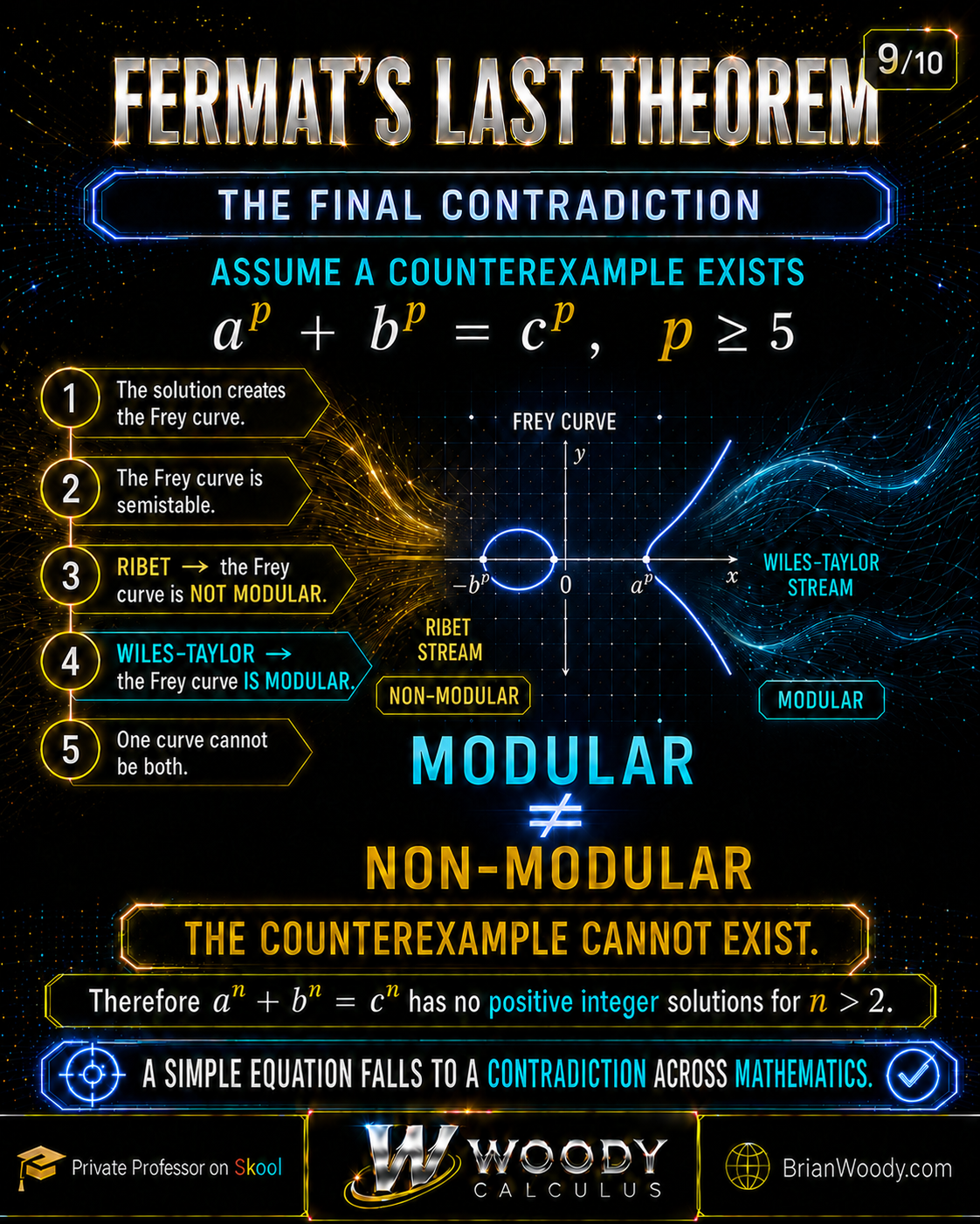
We can now complete the proof developed across the preceding eight parts.
Assume Fermat’s Last Theorem is false. Then for some prime \(p\ge5\), there is a primitive solution
a^p+b^p=c^p.
\]
Construct the Frey curve
E_{a,b,p}:y^2=x(x-a^p)(x+b^p).
\]
Frey and Hellegouarch
The hypothetical solution creates a highly constrained semistable elliptic curve.
Serre and Ribet
If the Frey curve were modular, level lowering would force its mod-\(p\) representation to arise from
S_2(\Gamma_0(2)).
\]
But
S_2(\Gamma_0(2))=\{0\}.
\]
Therefore
E_{a,b,p}\text{ is not modular}.
\]
Wiles and Taylor
Every semistable elliptic curve over \(\mathbb Q\) is modular. Therefore
E_{a,b,p}\text{ is modular}.
\]
The same curve cannot be both modular and non-modular:
\begin{aligned}
E_{a,b,p}\text{ modular}
\qquad\text{and}\qquad
E_{a,b,p}\text{ non-modular}
\end{aligned}
\]
is impossible.
The contradiction came only from assuming that the Fermat solution exists. Therefore no such solution exists.
\boxed{
a^n+b^n=c^n,
\quad n>2,
\quad abc\ne0
\quad\text{has no integer solutions.}
}
\]
Fermat’s Last Theorem is proved.
The Proof in One Unbroken Chain
The full logical spine is now visible:
\begin{aligned}
a^p+b^p=c^p
&\Longrightarrow
E_{a,b,p}\text{ semistable},\\
E_{a,b,p}\text{ modular}
&\overset{\text{Ribet}}{\Longrightarrow}
\bar\rho_{E,p}\text{ arises at level }2,\\
S_2(\Gamma_0(2))=0
&\Longrightarrow
E_{a,b,p}\text{ not modular},\\
\bar\rho\text{ modular}
&\overset{R=\mathbf T}{\Longrightarrow}
\rho\text{ modular},\\
\text{Langlands–Tunnell}+\text{3–5 trick}
&\Longrightarrow
\text{every semistable }E/\mathbb Q\text{ modular},\\
E_{a,b,p}\text{ semistable}
&\Longrightarrow
E_{a,b,p}\text{ modular},\\
\text{modular and non-modular}
&\Longrightarrow
\bot.
\end{aligned}
\]
Every arrow has now been explained rather than hidden behind “advanced mathematics.”
What Wiles Proved—and What Came Later
The 1995 theorem proves that every semistable elliptic curve over \(\mathbb Q\) is modular. That is exactly the case needed for the Frey curve and Fermat’s Last Theorem.
It did not yet prove modularity for every elliptic curve over \(\mathbb Q\), because elliptic curves with additive reduction fall outside the semistable class.
The full modularity theorem was completed through subsequent work, culminating in the 2001 theorem of Christophe Breuil, Brian Conrad, Fred Diamond, and Richard Taylor:
\boxed{
\text{Every elliptic curve over }\mathbb Q\text{ is modular.}
}
\]
The Taylor–Wiles method also became far more than a tool for one famous theorem. Its descendants drive modern modularity lifting, automorphy lifting, and major portions of the Langlands program.
The proof of Fermat’s Last Theorem solved a 358-year-old problem and simultaneously created machinery for problems mathematicians had not yet been able to formulate fully.
Part IX — Elliptic Curves in Cryptography: From the Group Law to Bitcoin
The proof of Fermat’s Last Theorem is now complete. We follow one of its central mathematical objects into a different world.
The elliptic curves in Wiles’s proof are studied over the rational numbers:
E/\mathbb Q.
\]
Their reductions modulo primes, their Galois representations, and their relationship with modular forms reveal deep arithmetic structure.
Elliptic-curve cryptography begins instead with a carefully chosen curve over a finite field:
E/\mathbb F_p.
\]
Its finite group of points becomes a computational platform. Repeated addition is fast. Reversing repeated addition appears to be hard. That asymmetry supports public keys, shared secrets, and digital signatures.
The connection is genuine—but it must be stated precisely.
Bitcoin does not use Wiles’s modularity-lifting theorem. It does not use the Frey curve. A Bitcoin node does not compute modular forms, deformation rings, Hecke algebras, or Galois cohomology when it verifies a transaction.
What Bitcoin does use is elliptic-curve arithmetic over a finite field, specifically the curve called secp256k1. The same broad mathematical species appears in both stories, but the arithmetic questions are different:
\boxed{
\begin{array}{c}
\text{Wiles: classify and compare arithmetic representations}\\[4pt]
\text{Cryptography: compute in a finite group while hiding a scalar}
\end{array}
}
\]
This part builds that second story from the ground up, derives the main formulas, works through a complete toy example, explains Bitcoin’s use of ECDSA and Schnorr signatures, and then reconnects the cryptography to the arithmetic geometry without blurring the boundary between them.
Direct Answer: How Are Elliptic Curves Used in Cryptography?
Elliptic-curve cryptography uses the finite abelian group formed by the points on an elliptic curve over a finite field. A private key is a secret integer \(d\), and the corresponding public key is the point
Q=dG,
\]
obtained by adding a public base point \(G\) to itself \(d\) times. Computing \(Q\) from \(d\) is fast, but recovering \(d\) from \(G\) and \(Q\) is the elliptic-curve discrete logarithm problem. Properly chosen parameters make the best known classical attacks computationally infeasible. Protocols use this one-way structure for key agreement and digital signatures.
The sentence “ECC is used for encryption” is sometimes acceptable as broad shorthand, but it hides important distinctions. Elliptic curves can support:
- Key agreement, such as elliptic-curve Diffie–Hellman, which helps two parties derive shared keying material.
- Digital signatures, such as ECDSA and Schnorr signatures, which authenticate messages and authorize actions.
- Integrated encryption constructions, which combine elliptic-curve key establishment with symmetric encryption and authentication.
Bitcoin primarily uses elliptic-curve digital signatures to authorize spending. Bitcoin’s public ledger is not made confidential by secp256k1.
One Equation, Different Number Systems
A short Weierstrass equation has the familiar form
E:y^2=x^3+ax+b.
\]
Over the real numbers, its solutions form one or two smooth components that we can draw as continuous curves. Over a finite field \(\mathbb F_p\), there is no continuous graph. The coordinates are residue classes
0,1,2,\ldots,p-1,
\]
and every operation is performed modulo \(p\).
The finite set of points is
E(\mathbb F_p)
=
\left\{(x,y)\in\mathbb F_p^2:
y^2\equiv x^3+ax+b\pmod p
\right\}
\cup\{\mathcal O\},
\]
where \(\mathcal O\) is the point at infinity.
The nonsingularity condition becomes
4a^3+27b^2\not\equiv0\pmod p.
\]
If this condition failed, the curve could have a cusp or crossing, and the clean group law required by the cryptographic construction would break down.
What survives after reduction modulo \(p\)?
Several structural features remain:
- each point \(P=(x,y)\) has an inverse \(-P=(x,-y)\);
- there is an identity element \(\mathcal O\);
- points can be added associatively;
- scalar multiplication \(dP\) means repeated addition;
- the full point set is a finite abelian group.
What changes is the geometry. Over \(\mathbb R\), slope formulas describe an actual line meeting an actual curve. Over \(\mathbb F_p\), those formulas are algebraic rules in modular arithmetic. A finite-field plot is a cloud of isolated points, not a smooth arc.
Hasse’s theorem keeps the group near size \(p\)
If
N_p=\#E(\mathbb F_p),
\]
then Hasse’s theorem states
\left|N_p-(p+1)\right|\le2\sqrt p.
\]
Equivalently,
N_p=p+1-a_p
\]
with
|a_p|\le2\sqrt p.
\]
The integer \(a_p\) is the trace of Frobenius. That name should now sound familiar: for an elliptic curve over \(\mathbb Q\), these traces appear in its \(L\)-function, its Galois representations, and the Fourier coefficients of the modular form attached to it.
This is our first authentic bridge:
\boxed{
a_p=p+1-\#E(\mathbb F_p)
}
\]
appears in the modularity story because it records arithmetic information across many primes. In cryptography, the size and subgroup structure of one selected finite group determine whether a chosen curve is suitable for secure computation.
The Group Law Over a Prime Field
Let
E:y^2=x^3+ax+b
\]
be nonsingular over \(\mathbb F_p\), where \(p>3\) is prime.
Identity and inverse
The point at infinity satisfies
P+\mathcal O=P.
\]
For
P=(x,y),
\]
the inverse is
-P=(x,-y\bmod p).
\]
Therefore
P+(-P)=\mathcal O.
\]
Adding two distinct nonopposite points
Let
P=(x_1,y_1),
\qquad
Q=(x_2,y_2),
\]
with \(P\ne Q\) and \(x_1\ne x_2\). Define
\lambda
=
(y_2-y_1)(x_2-x_1)^{-1}\pmod p.
\]
Then
x_3=\lambda^2-x_1-x_2\pmod p,
\]
y_3=\lambda(x_1-x_3)-y_1\pmod p,
\]
and
P+Q=(x_3,y_3).
\]
Doubling a point
If \(P=Q\) and \(y_1\ne0\), define
\lambda
=
(3x_1^2+a)(2y_1)^{-1}\pmod p.
\]
Then use the same coordinate formulas:
x_3=\lambda^2-2x_1\pmod p,
\]
y_3=\lambda(x_1-x_3)-y_1\pmod p.
\]
If \(y_1=0\), the tangent is vertical and
2P=\mathcal O.
\]
“Division” means a modular inverse
The expression
\frac{y_2-y_1}{x_2-x_1}
\]
does not mean ordinary real-number division. It means
(y_2-y_1)(x_2-x_1)^{-1}\pmod p,
\]
where \((x_2-x_1)^{-1}\) is the unique nonzero residue satisfying
(x_2-x_1)(x_2-x_1)^{-1}\equiv1\pmod p.
\]
Because \(p\) is prime, every nonzero element of \(\mathbb F_p\) has a multiplicative inverse. The extended Euclidean algorithm can compute it efficiently.
This is the exact moment where the geometric chord-and-tangent picture becomes a computational group operation.
A Complete Toy Curve: \(y^2=x^3+2x+2\pmod{17}\)
To see the machinery without 256-bit integers, consider
E:y^2=x^3+2x+2\pmod{17}.
\]
Its discriminant factor is nonzero:
4(2)^3+27(2)^2
=32+108
=140
\equiv4\pmod{17}.
\]
So the curve is nonsingular.
Take
G=(5,1).
\]
It lies on the curve because
1^2
\equiv
5^3+2(5)+2
=137
\equiv1\pmod{17}.
\]
Compute \(2G\)
For doubling,
\lambda
=(3\cdot5^2+2)(2\cdot1)^{-1}\pmod{17}.
\]
Now
3\cdot25+2=77\equiv9\pmod{17},
\]
and
2^{-1}\equiv9\pmod{17}
\]
because \(2\cdot9=18\equiv1\pmod{17}\). Therefore
\lambda\equiv9\cdot9=81\equiv13\pmod{17}.
\]
Then
x_{2G}
\equiv13^2-2(5)
\equiv169-10
\equiv6\pmod{17},
\]
and
y_{2G}
\equiv13(5-6)-1
\equiv-14
\equiv3\pmod{17}.
\]
Thus
2G=(6,3).
\]
Compute \(3G\)
Add \(2G=(6,3)\) and \(G=(5,1)\):
\lambda
\equiv
(1-3)(5-6)^{-1}
\equiv(-2)(-1)^{-1}
\equiv2\pmod{17}.
\]
Therefore
x_{3G}\equiv2^2-6-5\equiv10\pmod{17},
\]
y_{3G}\equiv2(6-10)-3\equiv6\pmod{17}.
\]
So
3G=(10,6).
\]
The complete cyclic subgroup
Repeated addition gives:
| \(k\) | \(kG\) | \(k\) | \(kG\) |
|---|---|---|---|
| 1 | \((5,1)\) | 10 | \((7,11)\) |
| 2 | \((6,3)\) | 11 | \((13,10)\) |
| 3 | \((10,6)\) | 12 | \((0,11)\) |
| 4 | \((3,1)\) | 13 | \((16,4)\) |
| 5 | \((9,16)\) | 14 | \((9,1)\) |
| 6 | \((16,13)\) | 15 | \((3,16)\) |
| 7 | \((0,6)\) | 16 | \((10,11)\) |
| 8 | \((13,7)\) | 17 | \((6,14)\) |
| 9 | \((7,6)\) | 18 | \((5,16)=-G\) |
| 19 | \(\mathcal O\) |
The point \(G\) has prime order
n=19.
\]
In fact, this curve has exactly 19 points, so \(G\) generates the whole group:
E(\mathbb F_{17})\cong\mathbb Z/19\mathbb Z.
\]
This toy group is far too small for security, but it contains the full algebraic skeleton of real elliptic-curve cryptography.
Scalar Multiplication: Easy Forward, Hard Backward
For an integer \(d\), scalar multiplication is
dG=\underbrace{G+G+\cdots+G}_{d\text{ times}}.
\]
No practical implementation performs \(d-1\) additions when \(d\) is enormous. It uses the binary expansion of \(d\).
For example,
13=8+4+1,
\]
so
13G=8G+4G+G.
\]
Repeated doubling computes
2G,\quad4G,\quad8G,
\]
and then selected points are added. This double-and-add method uses only \(O(\log d)\) group operations.
On the toy curve,
8G=(13,7),
\qquad
4G=(3,1),
\]
and the result is
13G=(16,4).
\]
The elliptic-curve discrete logarithm problem
Now reverse the question.
Given
G=(5,1)
\]
and
Q=(16,4),
\]
find \(d\) such that
Q=dG.
\]
On our 19-element group, we can inspect the table and discover
d=13.
\]
For a cryptographic group whose prime-order subgroup has roughly \(2^{256}\) elements, listing the multiples is impossible in practice.
The computational problem is:
\boxed{
\text{Given }G\text{ and }Q=dG,\text{ recover }d.
}
\]
That is the elliptic-curve discrete logarithm problem, or ECDLP.
Why a 256-bit group offers about 128 bits of classical security
Generic classical attacks such as Pollard’s rho method require on the order of
\sqrt n
\]
group operations when the relevant subgroup has order \(n\).
If
n\approx2^{256},
\]
then
\sqrt n\approx2^{128}.
\]
So “256-bit elliptic-curve key” does not mean “256 bits of security.” The standard estimate is approximately 128 bits of classical security.
The security claim is not that reversing scalar multiplication is logically impossible. It is that, for a well-chosen curve and the best publicly known classical methods, the required computation is infeasible.
The historical leap
In the mid-1980s, Victor Miller and Neal Koblitz independently proposed using elliptic-curve groups for public-key cryptography. The crucial insight was not merely that elliptic curves form groups. Mathematicians had known that for generations.
The leap was to recognize that these groups offered:
- efficient arithmetic;
- compact public keys;
- a discrete-logarithm problem without the subexponential attacks known for some more classical finite-field groups;
- a flexible platform for adapting established public-key ideas.
Arithmetic geometry had become computational infrastructure.
Private Keys and Public Keys
Choose public domain parameters
(p,a,b,G,n,h),
\]
where:
- \(p\) defines the field \(\mathbb F_p\);
- \(a\) and \(b\) define the curve;
- \(G\) is a public base point;
- \(n\) is the order of \(G\);
- \(h=\#E(\mathbb F_p)/n\) is the cofactor.
A private key is an integer
d\in\{1,2,\ldots,n-1\}.
\]
The public key is
Q=dG.
\]
The private key is not a point. It is a scalar. The public key is a curve point—or, in an encoding, enough information to recover the intended point.
The public key can be distributed openly because computing \(d\) from \(Q=dG\) is believed hard. But the public key does not automatically establish a person’s identity. A protocol also needs a trustworthy way to associate the key with an account, certificate, script condition, device, or other identity claim.
Digital Signatures Are Not Encryption
A digital signature answers a different question from encryption.
Encryption asks
Who can read this information?
A digital signature asks
Did a holder of the private key authorize this exact message?
A secure digital-signature scheme aims to provide message integrity and authenticity. Anyone with the public key can verify a signature, but they cannot efficiently create a valid signature on a new message without the private key.
Bitcoin’s ledger is intentionally public. Elliptic-curve signatures do not hide transaction amounts or recipients. They provide cryptographic evidence that a transaction satisfies a key-based spending condition.
This distinction eliminates one of the most common statements in popular explanations:
\boxed{
\text{Bitcoin uses elliptic curves primarily for authorization, not secrecy.}
}
\]
ECDSA: The Elliptic Curve Digital Signature Algorithm
Let:
- \(G\) be a base point of prime order \(n\);
- \(d\) be the signer’s private key;
- \(Q=dG\) be the public key;
- \(z\) be the integer derived from the message hash.
Signing
To sign, the signer chooses a secret per-signature nonce
k\in\{1,2,\ldots,n-1\}.
\]
Then:
- Compute \[
R=kG=(x_R,y_R).
\] - Set \[
r=x_R\bmod n.
\] - Compute \[
s=k^{-1}(z+rd)\pmod n.
\] - If \(r=0\) or \(s=0\), choose a new nonce and repeat.
The signature is
(r,s).
\]
Verifying
The verifier first checks
1\le r,s\le n-1.
\]
Then compute
w=s^{-1}\pmod n,
\]
u_1=zw\pmod n,
\qquad
u_2=rw\pmod n,
\]
and
X=u_1G+u_2Q.
\]
The signature is accepted when \(X\ne\mathcal O\) and
x_X\bmod n=r.
\]
Why verification works
From the signing equation,
s=k^{-1}(z+rd)\pmod n.
\]
Multiply by \(k\):
sk=z+rd\pmod n.
\]
Now multiply by \(s^{-1}\):
k=zs^{-1}+rds^{-1}\pmod n.
\]
Multiplying the scalar identity by \(G\) gives
kG
=
(zs^{-1})G+(rs^{-1})(dG).
\]
Because \(Q=dG\),
R=u_1G+u_2Q=X.
\]
Therefore the verifier reconstructs the same ephemeral point’s \(x\)-coordinate without learning either \(d\) or \(k\).
A Complete Toy ECDSA Signature
Continue with the group generated by
G=(5,1)
\]
of order
n=19.
\]
Choose the private key
d=7.
\]
Then the public key is
Q=7G=(0,6).
\]
Suppose the message hash has been converted to
z=9,
\]
and choose the nonce
k=5.
\]
Sign
First,
R=5G=(9,16),
\]
so
r=9.
\]
Because
5^{-1}\equiv4\pmod{19},
\]
we have
\begin{aligned}
s
&\equiv5^{-1}(9+9\cdot7)\pmod{19}\\
&\equiv4(72)\pmod{19}\\
&\equiv4(15)\pmod{19}\\
&\equiv3\pmod{19}.
\end{aligned}
\]
The signature is
(r,s)=(9,3).
\]
Verify
Compute
w=3^{-1}\equiv13\pmod{19}.
\]
Then
u_1=9(13)\equiv3\pmod{19},
\]
and
u_2=9(13)\equiv3\pmod{19}.
\]
Therefore
\begin{aligned}
X
&=3G+3Q\\
&=3G+3(7G)\\
&=24G\\
&=5G\\
&=(9,16).
\end{aligned}
\]
Its \(x\)-coordinate is 9, matching \(r\). The signature verifies.
This example is not secure—the group is tiny, and we deliberately exposed the nonce. It is a transparent model of the real algebra.
The Nonce Is a One-Time Secret
ECDSA has a dangerous feature: the nonce \(k\) is mathematically entangled with the private key. Reuse it, bias it, predict it, or leak enough side-channel information about it, and the long-term private key may be recoverable.
Suppose the same nonce \(k\) signs two different message hashes \(z_1\) and \(z_2\), producing
s_1=k^{-1}(z_1+rd)\pmod n
\]
and
s_2=k^{-1}(z_2+rd)\pmod n.
\]
Subtract:
s_1-s_2=k^{-1}(z_1-z_2)\pmod n.
\]
Therefore
\boxed{
k=(z_1-z_2)(s_1-s_2)^{-1}\pmod n.
}
\]
Once \(k\) is known,
\boxed{
d=(s_1k-z_1)r^{-1}\pmod n.
}
\]
Watch the toy key collapse
Our first signature used
z_1=9,
\qquad
(r,s_1)=(9,3),
\qquad
k=5.
\]
Suppose the same nonce signs a second hash
z_2=4.
\]
Then
s_2
\equiv5^{-1}(4+9\cdot7)
\equiv2\pmod{19}.
\]
An observer sees the two signatures and computes
k
\equiv
(9-4)(3-2)^{-1}
\equiv5\pmod{19}.
\]
Then
\begin{aligned}
d
&\equiv(3\cdot5-9)9^{-1}\pmod{19}\\
&\equiv6\cdot17\pmod{19}\\
&\equiv7\pmod{19}.
\end{aligned}
\]
The private key is recovered exactly.
Deterministic ECDSA helps, but does not solve everything
RFC 6979 specifies deterministic nonce generation from the private key and the message hash. This removes dependence on obtaining fresh random bits for each ECDSA signature and prevents ordinary accidental nonce reuse when implemented correctly.
It does not make careless implementations safe. Constant-time arithmetic, protected memory, correct message processing, fault resistance, and side-channel defenses still matter. The RFC itself warns that deterministic behavior can interact with side-channel attacks.
Cryptography is not merely a theorem about a group. It is the theorem plus a precise protocol plus a hardened implementation plus secure key custody.
The Curve secp256k1
Bitcoin uses the prime-field curve called
\texttt{secp256k1}.
\]
The name encodes its origin:
- sec: Standards for Efficient Cryptography;
- p: a curve over a prime field \(\mathbb F_p\);
- 256: the field size is approximately 256 bits;
- k: parameters associated with a Koblitz-type curve in SEC terminology;
- 1: the first curve in that named family and size.
Field prime
p=2^{256}-2^{32}-977.
\]
In hexadecimal,
\texttt{FFFFFFFFFFFFFFFFFFFFFFFFFFFFFFFFFFFFFFFFFFFFFFFFFFFFFFFEFFFFFC2F}.
\]
Curve equation
E:y^2=x^3+7\pmod p.
\]
Thus
a=0,
\qquad
b=7.
\]
The nonsingularity condition is immediate because
4a^3+27b^2=27\cdot49\not\equiv0\pmod p.
\]
Base point
The standard base point \(G=(x_G,y_G)\) has coordinates
x_G=
\texttt{79BE667EF9DCBBAC55A06295CE870B07029BFCDB2DCE28D959F2815B16F81798},
\]
y_G=
\texttt{483ADA7726A3C4655DA4FBFC0E1108A8FD17B448A68554199C47D08FFB10D4B8}.
\]
Subgroup order
The order of \(G\) is the prime
n=
\texttt{FFFFFFFFFFFFFFFFFFFFFFFFFFFFFFFEBAAEDCE6AF48A03BBFD25E8CD0364141}.
\]
Cofactor
h=1.
\]
Because the cofactor is 1,
\#E(\mathbb F_p)=n,
\]
and every nonidentity point lies in the same prime-order group generated by \(G\).
Security scale
The order \(n\) is close to \(2^{256}\). Generic classical discrete-logarithm attacks therefore have a work factor on the order of
2^{128}.
\]
The special form of the field prime and the curve’s efficiently computable endomorphism support fast legitimate arithmetic. They do not turn the private-key problem into an easy classical computation.
secp256k1 is not NIST P-256
The similarly sized curve commonly called NIST P-256 is also known as secp256r1. It is a different curve with different coefficients, base point, order, and parameter-generation history.
The labels are easy to confuse:
\texttt{secp256k1}\ne\texttt{secp256r1}.
\]
Bitcoin uses secp256k1.
How Bitcoin Uses Elliptic-Curve Keys
The phrase “your bitcoin is stored in your wallet” is a useful interface metaphor, not a literal description of the protocol.
Bitcoin’s ledger records transaction outputs. Each unspent transaction output, or UTXO, is locked by a script condition. A wallet manages the keys and data needed to construct a transaction that satisfies those conditions.
The coins are not little files inside the wallet. The wallet protects authorization material.
A simplified key-based spending flow
- A wallet generates a private scalar \(d\).
- It computes a public point \[
Q=dG.
\] - A transaction output commits to a key or to a script condition involving a key.
- To spend, the wallet constructs the precise transaction message required by the applicable signature-hash rules.
- It signs that message with the private key.
- Network nodes verify the signature and every other consensus condition.
- A valid signature shows that the transaction satisfies the specified key condition; it does not override script rules, prevent double-spending by itself, or guarantee transaction inclusion.
Public key is not always the address
Depending on the output type, a Bitcoin address may encode:
- a hash of a public key;
- a hash of a script;
- a witness program;
- a Taproot output key.
An address is a human-facing encoding of payment instructions. It should not be universally defined as “the public key.”
For traditional compressed public keys, SEC point encoding stores the \(x\)-coordinate plus one bit indicating which of the two possible \(y\)-coordinates is intended. This gives a 33-byte encoding rather than storing both 32-byte coordinates.
ECDSA in traditional Bitcoin spending
Bitcoin traditionally used ECDSA over secp256k1 for transaction authorization, and ECDSA remains part of the protocol for legacy and SegWit version 0 spending paths.
The transaction-specific details matter. The “message” is not simply a sentence or the visual summary shown by a wallet. It is a hash derived from a precisely serialized transaction context under the selected signature-hash mode.
A signature can only be interpreted correctly inside those consensus rules.
Schnorr Signatures: A Cleaner Linear Equation
An idealized elliptic-curve Schnorr signature begins with:
- private key \(d\);
- public key \(P=dG\);
- nonce \(k\);
- nonce point \(R=kG\);
- message \(m\).
Compute a challenge
e=H(R\,\|\,P\,\|\,m)\pmod n,
\]
and a response
s=k+ed\pmod n.
\]
The signature verifies because
\begin{aligned}
sG
&=(k+ed)G\\
&=kG+e(dG)\\
&=R+eP.
\end{aligned}
\]
So the verification equation is
\boxed{sG=R+eP.}
\]
This linearity is one of Schnorr signatures’ great attractions. It supports efficient reasoning about key aggregation, multisignature protocols, threshold constructions, and batch verification—provided those higher-level protocols are designed correctly.
Linearity is powerful, not automatically safe. Naively adding keys or nonces can create rogue-key and nonce-manipulation attacks. Secure multiparty schemes need their own proofs, commitments, coefficient rules, transcript binding, and nonce discipline.
BIP 340 Schnorr Signatures on secp256k1
Bitcoin’s BIP 340 specifies 64-byte Schnorr signatures over the same secp256k1 curve used for ECDSA.
Its exact byte-level rules matter because consensus systems cannot tolerate two honest implementations disagreeing about whether a signature is valid.
X-only public keys
For a given valid \(x\)-coordinate on secp256k1, there are normally two points:
(x,y)
\qquad\text{and}\qquad
(x,-y).
\]
BIP 340 chooses the point with even \(y\). Therefore a public key can be encoded with only the 32-byte \(x\)-coordinate.
If the original public point
P=d^{\prime}G
\]
has odd \(y\), signing uses the equivalent scalar
d=n-d^{\prime}
\]
so that \(dG=-P\) has the same \(x\)-coordinate and even \(y\).
Tagged hashes
BIP 340 uses domain-separated tagged hashes. Schematically,
H_{\text{tag}}(x)
=
\operatorname{SHA256}
\bigl(
\operatorname{SHA256}(\text{tag})
\,\|\,
\operatorname{SHA256}(\text{tag})
\,\|\,
x
\bigr).
\]
Different tags separate auxiliary randomness, nonce derivation, and the signature challenge.
Signing structure
BIP 340 derives a nonce scalar \(k^{\prime}\) from the secret key, public key, message, and auxiliary data. If
R=k^{\prime}G
\]
has odd \(y\), it replaces \(k^{\prime}\) by
k=n-k^{\prime}.
\]
Then \(R=kG\) has even \(y\).
The challenge is
e
=
H_{\texttt{BIP0340/challenge}}
(r\,\|\,P_x\,\|\,m)
\pmod n,
\]
where
r=x_R.
\]
The response is
s=k+ed\pmod n.
\]
The 64-byte signature is the concatenation of the 32-byte encodings of \(r\) and \(s\).
Verification structure
The verifier reconstructs
R=sG-eP.
\]
It accepts only if:
- the public key lifts to a valid even-\(y\) curve point;
- \(r<p\) and \(s<n\);
- \(R\ne\mathcal O\);
- \(R\) has even \(y\);
- \(x_R=r\).
These are not decorative encoding decisions. They make the scheme unambiguous at the byte level.
Taproot: Where Bitcoin Uses BIP 340
BIP 341 defines Taproot as a SegWit version 1 output type. A Taproot output combines:
- a public-key spending condition;
- zero or more script conditions organized through a Merkle tree.
The output commits to a tweaked public key. A spend can use:
- a key path, presenting a BIP 340 Schnorr signature; or
- a script path, revealing the selected script, the data needed to satisfy it, and a Merkle proof connecting it to the committed tree.
When the key path is used, unused script alternatives remain hidden. This can improve efficiency and avoid revealing unnecessary spending conditions.
A Taproot key-path signature is a 64-byte BIP 340 Schnorr signature, optionally followed by a signature-hash byte when the default mode is not implied.
ECDSA and Schnorr coexist
It would be wrong to say, without qualification, “Bitcoin replaced ECDSA with Schnorr.”
The accurate statement is:
- legacy and SegWit version 0 spending paths use ECDSA over secp256k1;
- Taproot’s version 1 key and signature rules use BIP 340 Schnorr signatures over secp256k1.
The same curve supports two different signature schemes.
What a Bitcoin Signature Proves—and What It Does Not
A valid signature can establish that a transaction message was authorized under a specified public key. It does not, by itself, prove:
- the signer’s legal identity;
- the signer’s moral or legal ownership of the funds;
- that the private key was not stolen;
- that the transaction obeys every other script rule;
- that the input has not already been spent;
- that miners will include the transaction;
- that the chain containing it will remain the accepted chain;
- that the transaction data are secret.
Bitcoin combines signatures with transaction structure, scripts, UTXO validation, a replicated ledger, proof of work, and consensus rules.
The white paper’s phrase “a chain of digital signatures” captures an essential part of the ownership-transfer model, but the system also needs a mechanism to establish a public ordering and prevent double-spending.
Elliptic curves solve the authorization problem. They do not solve the entire distributed-consensus problem.
Implementation Security: Where Beautiful Algebra Meets Hostile Reality
A mathematically sound curve can be deployed insecurely. Real attacks often target implementations and key handling rather than the abstract ECDLP.
1. Weak or reused nonces
ECDSA nonce reuse reveals the private key algebraically. Partial nonce bias or leakage can also enable lattice or side-channel attacks.
BIP 340’s default signing algorithm derives a synthetic nonce using the secret key, public key, message, and auxiliary data. The auxiliary randomness improves resistance to certain fault and side-channel attacks, but implementers must follow the specification exactly.
2. Timing, cache, power, and electromagnetic leakage
Secret-dependent branches, table lookups, or memory access patterns may leak information about \(d\) or \(k\).
Operations involving secret scalars should be constant-time and avoid secret-dependent memory access as far as the platform and threat model require.
3. Fault injection
An attacker who can alter a computation, voltage, clock, or memory value may produce faulty outputs that reveal secrets. Verification after signing and redundant checks can be part of a defense.
4. Invalid points and unvalidated inputs
Key-agreement protocols must validate public inputs according to their standards. Invalid-curve and small-subgroup attacks exploit arithmetic performed on malicious points or groups.
secp256k1’s cofactor \(h=1\) simplifies subgroup concerns for valid curve points, but it does not justify accepting malformed encodings or skipping all validation in every protocol.
5. Key storage and backups
No discrete-log attack is needed if an attacker can read the seed phrase, private key, signing device memory, cloud backup, clipboard, or recovery photograph.
The system’s effective security is bounded by its weakest key-custody path.
6. Supply-chain and dependency risk
A correct cryptographic library can be undermined by a compromised build, malicious dependency, unsafe wrapper, incorrect random-number generator, or misuse of the API.
Bitcoin Core’s libsecp256k1 project is designed as a high-performance, high-assurance C library for secp256k1 operations. Its documented features include ECDSA, BIP 340 Schnorr signatures, deterministic ECDSA nonce generation, efficient verification, and constant-time secret-key operations. That is an example of the level of engineering cryptographic arithmetic demands—not permission to copy formulas into production code.
The rule for learners and implementers
Write toy code to understand the mathematics.
Use reviewed, purpose-appropriate cryptographic libraries for real secrets.
Quantum Computers and the ECDLP
The classical security of secp256k1 rests on the apparent difficulty of the elliptic-curve discrete logarithm problem.
Peter Shor showed that a sufficiently capable quantum computer could solve discrete logarithms in polynomial time. The theoretical threat therefore applies to elliptic-curve systems as well as to several other familiar public-key systems.
This does not mean that someone can run a short program on an ordinary computer and recover a Bitcoin private key. Shor’s algorithm requires a large, fault-tolerant quantum computation capable of operating on the relevant cryptographic instance.
The durable conclusion is:
\boxed{
\text{ECDLP is hard for known classical methods but not post-quantum secure.}
}
\]
Post-quantum cryptography uses different mathematical problems designed to resist both classical and quantum attacks. NIST finalized its first post-quantum standards in 2024, including standards for key establishment and digital signatures.
Predicting when—or whether—a quantum computer capable of attacking deployed 256-bit elliptic-curve systems will exist is an engineering forecast, not a theorem. The mathematical vulnerability and the practical timeline are separate questions.
secp256k1 Is Not the Frey Curve
The Frey curve associated with a hypothetical Fermat solution has the form
E_{a,b,p}:y^2=x(x-a^p)(x+b^p),
\]
up to equivalent choices and normalizations.
Its coefficients depend on the hypothetical integers \(a,b,p\). It is an elliptic curve over \(\mathbb Q\), studied through its discriminant, conductor, reduction behavior, and Galois representations.
secp256k1 is the fixed curve
y^2=x^3+7
\]
over the finite field determined by
p=2^{256}-2^{32}-977.
\]
Its parameters are public constants chosen for cryptographic computation.
They are not remotely the same curve:
| Feature | Frey curve | secp256k1 |
|---|---|---|
| Base setting | Curve over \(\mathbb Q\) | Curve over \(\mathbb F_p\) |
| Coefficients | Depend on a hypothetical Fermat solution | Fixed public constants \(a=0,b=7\) |
| Main role | Convert a Diophantine solution into arithmetic contradiction | Provide a finite group for keys and signatures |
| Central invariants | Discriminant, conductor, reduction, Galois representation | Field prime, base point, subgroup order, cofactor |
| Main theorem/problem | Modularity and level lowering | ECDLP hardness and protocol security |
| Used by Bitcoin? | No | Yes |
Calling both objects “elliptic curves” identifies a shared mathematical category. It does not make their purposes interchangeable.
Does Bitcoin Use the Mathematics of Wiles’s Proof?
The honest answer has two levels.
Direct operational answer: no
Bitcoin transaction validation does not invoke:
- the modularity theorem;
- the Taniyama–Shimura conjecture;
- Ribet’s level-lowering theorem;
- modular forms;
- Hecke operators or Hecke algebras;
- deformation rings;
- Selmer groups;
- Taylor–Wiles patching.
No step in BIP 340 asks whether secp256k1 is modular. No ECDSA verifier computes an \(L\)-function. Fermat’s Last Theorem is not a security assumption of Bitcoin.
Deeper mathematical answer: they inhabit connected arithmetic geometry
The stories share foundational structures:
- Elliptic-curve group laws. Both begin with curves carrying an abelian group structure.
- Finite-field reductions. Wiles’s world studies how a rational curve behaves modulo many primes; cryptography computes inside one selected finite-field group.
- Frobenius. Point counts determine traces \(a_p\), which feed the Galois and modular sides of the modularity story.
- Torsion and Galois action. The points of order \(\ell\) on an elliptic curve form the representation space \[
E[\ell]\cong(\mathbb Z/\ell\mathbb Z)^2
\] used in modularity arguments. Cryptographic protocols instead select a large cyclic subgroup and hide a scalar in it. - Arithmetic algorithms. Point addition, scalar multiplication, finite fields, inversion, and group order are central to explicit computation in both arithmetic geometry and cryptography.
The overlap is conceptual and structural. The proof techniques and computational goals are different.
The Most Important Comparison in the Entire Lesson
| Question | Fermat–Wiles world | Elliptic-curve cryptography |
|---|---|---|
| Typical curve | \(E/\mathbb Q\) | \(E/\mathbb F_p\) |
| Prime behavior | Study reductions across many primes | Fix one finite field for the protocol |
| Main data | \(a_p\), conductor, \(L\)-function, Galois representations | \(p,a,b,G,n,h\), encoded points, scalars |
| Central operation | Compare arithmetic and automorphic representations | Scalar multiplication in a finite group |
| Hard problem | Prove modularity and control deformations | Recover \(d\) from \(Q=dG\) |
| Key tools | Modular forms, Hecke algebras, deformation theory, patching | Finite-field arithmetic, hash functions, protocol design, hardened code |
| Output | A theorem about elliptic curves and Fermat’s equation | Signatures, key agreement, authorization |
| Failure mode | Logical gap or unmet arithmetic hypothesis | Cryptanalytic break, nonce failure, side channel, key theft, consensus mismatch |
The comparison is more impressive when the differences remain visible.
Part X — Meaning, Myths, Personal Authority, and Mastery
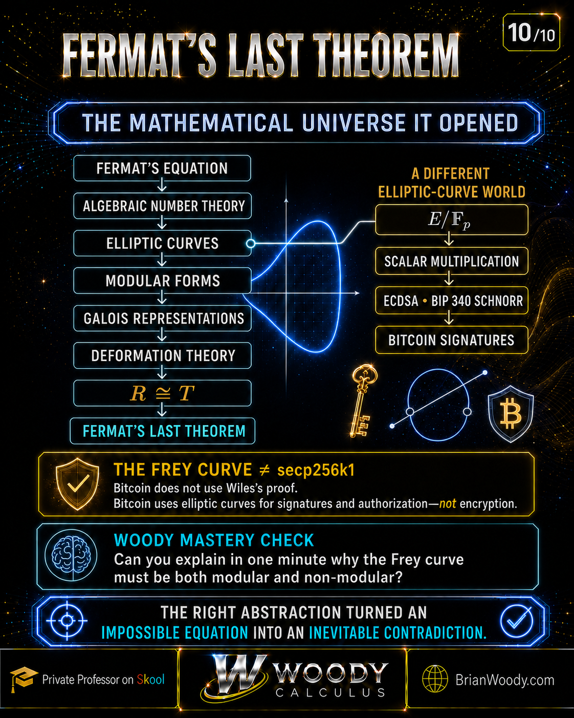
The Proof at Five Levels of Magnification
One reason explanations of Fermat’s Last Theorem often feel either vague or impossibly technical is that they remain at only one scale. The proof becomes clearer when we deliberately change magnification.
Level 1: The Diophantine statement
For every integer \(n>2\), there are no positive integers \(a,b,c\) satisfying
a^n+b^n=c^n.
\]
This level tells us exactly what must be proved.
Level 2: The contradiction through the Frey curve
A hypothetical solution creates a semistable elliptic curve. Ribet says that curve cannot be modular. Wiles says it must be modular. Contradiction.
This level tells us the global proof strategy.
Level 3: Matching arithmetic fingerprints
An elliptic curve \(E/\mathbb Q\) has point-count data
a_\ell(E)=\ell+1-\#E(\mathbb F_\ell)
\]
at primes of good reduction. A normalized weight-two newform
f(z)=\sum_{m=1}^{\infty}a_m(f)q^m
\]
has Hecke eigenvalues \(a_\ell(f)\).
The curve is modular when these arithmetic fingerprints agree:
a_\ell(E)=a_\ell(f)
\]
for the appropriate primes, equivalently when their \(L\)-functions match.
This level explains what “modular” means arithmetically.
Level 4: Galois representations carry the comparison
The \(\ell\)-power torsion of an elliptic curve produces a representation
\rho_{E,\ell}:
G_{\mathbb Q}\longrightarrow
\operatorname{GL}_2(\mathbb Z_\ell).
\]
Modular forms produce compatible Galois representations with the same Frobenius traces. Wiles’s strategy begins with a residual representation
\bar\rho:
G_{\mathbb Q}\longrightarrow
\operatorname{GL}_2(k)
\]
already known to be modular and asks whether an admissible \(\ell\)-adic lift \(\rho\) must also be modular.
This level explains how elliptic curves and modular forms can be compared inside the same language.
Level 5: The ring identity controls every lift at once
The universal deformation ring \(R\) parameterizes all admissible Galois lifts of \(\bar\rho\). The Hecke algebra \(\mathbf T\) parameterizes the modular lifts coming from Hecke eigenforms. There is a natural surjection
R\twoheadrightarrow\mathbf T.
\]
The possible kernel is the hiding place for admissible non-modular lifts. Proving
R\cong\mathbf T
\]
shows that every admissible lift is already modular.
Taylor–Wiles auxiliary primes and patching provide the depth and dimension control needed to eliminate the kernel.
This level explains the engine inside modularity lifting.
Why all five levels are necessary
Each level answers a different question:
| Level | Question answered |
|---|---|
| Diophantine equation | What is the theorem? |
| Frey contradiction | What is the proof strategy? |
| Arithmetic fingerprints | What does modularity mean? |
| Galois representations | What common language compares the objects? |
| \(R=\mathbf T\) | Why does one modular residual case control all allowed lifts? |
A strong explanation does not choose between the simple version and the deep version. It builds a staircase connecting them.
Why Fermat’s Last Theorem Mattered
Fermat’s Last Theorem is not important because engineers needed to know whether
a^{137}+b^{137}=c^{137}
\]
has positive-integer solutions.
Its importance is more profound.
1. The problem generated mathematics
Attempts to prove the theorem helped motivate or accelerate:
- infinite descent;
- arithmetic in algebraic number fields;
- the study of failures of unique factorization;
- ideal numbers and ideal theory;
- class groups and regular primes;
- increasingly systematic study of Diophantine equations;
- the decisive interaction among elliptic curves, modular forms, and Galois representations;
- modularity-lifting and patching techniques with influence far beyond FLT.
Even a failed attempt could expose the exact structure mathematics lacked.
3. The proof exemplified a local-to-global strategy
Wiles did not inspect every elliptic curve globally in one direct calculation. He imposed precise local conditions at primes, encoded global deformations in a universal ring, compared them with modular Hecke data, and used global duality and patching to control the whole space.
The global theorem is assembled from carefully synchronized local information.
4. The proof changed the target
Fermat’s equation was not defeated by manipulating it until a contradiction fell out. The proof asked a more powerful question:
What mathematical object would a counterexample force into existence?
Once the Frey curve is built, the original integers are no longer the main actors. The supposed solution has been translated into an object that mature theories can constrain.
This is a reusable problem-solving principle:
\boxed{
\text{When a problem resists attack, change the category in which it lives.}
}
\]
5. The proof demonstrated how mathematics corrects itself
The 1993 announcement was not the end of verification. A serious gap remained. The community’s scrutiny exposed it. Wiles and Taylor worked to repair it. The final proof used a different route for the crucial ring-theoretic step.
The gap is not an embarrassment to hide. It is one of the most illuminating parts of the story. Mathematics earns certainty through proof, criticism, revision, and reproducibility—not through reputation or applause.
Did Fermat Really Have a Proof?
No valid general proof by Fermat survives. Whether he once believed he had one is a historical question; whether an elementary proof exists is a mathematical question. Neither can be settled by confidence alone.
What the evidence supports
- Fermat wrote the famous marginal claim in his copy of Diophantus’s Arithmetica, conventionally dated around 1637, although the exact dating is not certain.
- The note says he had found a remarkable proof that the margin could not contain.
- His son Samuel published the annotations posthumously in 1670.
- No general proof appears in Fermat’s surviving papers or correspondence.
- Fermat circulated many results as challenges, but the full general claim does not reappear in the same sustained way.
- Fermat possessed an infinite-descent argument yielding the fourth-power case.
- The known proof uses mathematical structures developed centuries after Fermat.
What the evidence does not prove
The modern proof’s sophistication does not logically imply that no elementary proof can exist. A theorem may have two very different proofs. Nor can we prove a claim about every thought Fermat once had.
The responsible verdict is:
\boxed{
\text{Skepticism that Fermat had a correct general proof is strongly justified,}
\text{ but absolute historical certainty is not.}
}
\]
The most plausible mathematical interpretation
Fermat may have had a correct descent for \(n=4\), an incomplete idea for another exponent, or an argument that silently assumed a false factorization property. The history of FLT repeatedly shows how natural such assumptions can appear.
That remains informed speculation, not recovered proof.
Wiles did not reconstruct Fermat’s missing argument
Wiles proved a theorem Fermat could not have formulated:
Every semistable elliptic curve over \(\mathbb Q\) is modular.
Fermat’s Last Theorem follows as a corollary through the Frey curve and Ribet’s theorem.
Therefore the phrase “Wiles found the proof Fermat left out of the margin” is historically and mathematically misleading.
Who Proved Fermat’s Last Theorem?
The conventional answer is Andrew Wiles, with Richard Taylor playing an essential role in the repair. That answer is correct. It is not the whole intellectual genealogy.
A precise attribution map
| Person or community | Essential contribution |
|---|---|
| Pierre de Fermat | Stated the general claim and developed the descent argument behind the \(n=4\) case |
| Leonhard Euler | Advanced the cubic case and arithmetic in enlarged number systems; his published proof contains a gap that can be repaired using related ideas |
| Sophie Germain | Created a general auxiliary-prime strategy and transformed the study from isolated exponents toward families of exponents |
| Dirichlet and Legendre | Completed the exponent \(5\) case through complementary work |
| Gabriel Lamé | Proved the exponent \(7\) case and helped precipitate the 1847 factorization crisis |
| Ernst Kummer | Repaired failed factorization with ideal numbers and proved FLT for regular primes |
| Gerd Faltings | Proved the Mordell conjecture, giving finiteness of rational points on each fixed higher-genus Fermat curve, but not their absence |
| Yutaka Taniyama, Goro Shimura, André Weil, and others | Developed the modularity conjecture connecting elliptic curves with modular forms |
| Yves Hellegouarch | Studied elliptic curves arising from Fermat-type solutions before the decisive bridge was formalized |
| Gerhard Frey | Highlighted the extraordinary semistable curve a Fermat counterexample would create |
| Jean-Pierre Serre | Formulated the representation-theoretic level-lowering prediction that made Frey’s idea precise |
| Kenneth Ribet | Proved the needed level-lowering theorem, showing that semistable modularity would imply FLT |
| Langlands and Tunnell | Supplied the modularity theorem for suitable odd irreducible two-dimensional mod-3 representations used as Wiles’s residual seed |
| Barry Mazur and the deformation-theory lineage | Developed fundamental deformation, modular-curve, and Hecke-algebra tools underlying the modularity-lifting method |
| Andrew Wiles | Proved semistable modularity through modularity lifting, developed the \(R=\mathbf T\) strategy and 3–5 trick, and derived FLT |
| Richard Taylor and Andrew Wiles | Created the auxiliary-prime patching repair that established the crucial minimal ring-theoretic theorem |
| Reviewers and collaborators | Tested the argument, identified weaknesses, simplified components, and helped convert an announcement into verified mathematics |
| Breuil, Conrad, Diamond, and Taylor | Completed modularity for every elliptic curve over \(\mathbb Q\) after the semistable case needed for FLT |
Credit is not diminished by explaining the network. Wiles’s accomplishment becomes more impressive when we see which centuries of mathematics he successfully assembled—and which new machinery he had to create.
Abstraction Was the Solution, Not the Obstacle
Readers sometimes ask why a problem about whole-number powers needs objects as abstract as ideals, modular forms, Galois representations, and deformation rings.
The answer is that each abstraction repairs a specific limitation.
Ideals repair broken factorization
Lamé’s proposed strategy wanted to factor
x^p+y^p
\]
inside a cyclotomic integer ring and reason as though prime factorization behaved exactly as it does in \(\mathbb Z\).
It does not.
Kummer’s ideal numbers restore a form of unique factorization at the level of ideals. The abstraction does not move away from arithmetic. It preserves the arithmetic information that element factorization loses.
Elliptic curves package a Diophantine solution
The Frey curve
y^2=x(x-a^p)(x+b^p)
\]
turns the hypothetical integers into discriminant, conductor, reduction, torsion, and Galois data.
The curve is a compression device: one geometric object remembers the exact divisibility features that Ribet’s theorem can exploit.
Modular forms make symmetry arithmetic
A modular form is not introduced because its graph resembles the elliptic curve. Its Hecke eigenvalues encode arithmetic information that can match the curve’s Frobenius traces.
The surprising correspondence is
a_\ell(f)=\ell+1-\#E(\mathbb F_\ell).
\]
Symmetry on the complex upper half-plane and point counts over finite fields reveal the same arithmetic fingerprint.
Galois representations create a common language
Elliptic curves and modular forms are different kinds of objects. Their associated Galois representations are comparable matrix-valued records of arithmetic symmetry.
Instead of comparing a curve directly with a holomorphic function, the proof compares
\rho_{E,\ell}
\qquad\text{and}\qquad
\rho_{f,\ell}.
\]
Deformation rings control infinitely many possibilities
The universal deformation ring does not list every lift one by one. It represents the entire admissible family. The Hecke algebra organizes the modular family.
Proving
R=\mathbf T
\]
proves an infinite collection of modularity statements simultaneously.
The abstraction is efficient because it controls a whole space rather than a single example.
Woody’s Reflection: Why This Proof Captured Me
I studied the proof of Fermat’s Last Theorem in a year-long, two-semester course at the University of Wisconsin–Madison. That amount of time for a theorem stated in one sentence did not feel excessive. It revealed the real point of the subject.
The excitement was never merely that an old puzzle had finally been solved. It was watching one mathematical language transform into another.
You begin with
a^n+b^n=c^n,
\]
an equation that looks elementary enough to attack with clever algebra. Then the problem opens. Factorization leads to ideals. A hypothetical solution becomes an elliptic curve. Point counts become Frobenius traces. Torsion points become Galois representations. Modular forms produce the same representation-theoretic data. Finally, entire families of possible lifts are controlled by rings.
For me, Galois Theory is one of the most beautiful parts of the story. The subject begins as a way to understand symmetries among polynomial roots. Here it grows into a language that records how the absolute Galois group acts on elliptic-curve torsion. Abstract Algebra stops being a collection of definitions and becomes the carrier of arithmetic information.
That is what I want a serious student to feel in this lesson: abstraction is not fog placed between you and the problem. The right abstraction is a lens. It shows relationships that the original coordinates hide.
The year-long course also changed the scale at which I thought about proof. A theorem can have a short logical ending and still require generations to build the vocabulary that makes the ending possible. The last contradiction is only a few lines. Understanding why every arrow is valid is the achievement.
The story of the 1993 gap matters to me as a teacher. Mathematics does not ask us to pretend that strong work is perfect on the first attempt. It asks us to expose the reasoning, locate the exact failure, preserve what remains correct, and rebuild the unsupported step. Wiles’s persistence is inspiring precisely because verification mattered.
This is why Fermat’s Last Theorem belongs in the Woody Calculus library. It is not just a famous result to memorize. It is a guided tour through the way modern mathematics thinks: translate, connect, test, repair, and prove.
— Woody
Myth Versus Fact
| Myth | Fact |
|---|---|
| Fermat’s Last Theorem and Fermat’s Little Theorem are the same result. | FLT concerns the impossibility of \(a^n+b^n=c^n\) for \(n>2\). Fermat’s Little Theorem concerns congruences such as \(a^p\equiv a\pmod p\) for prime \(p\). |
| The theorem says the equation has no real solutions. | It has abundant real solutions. FLT rules out positive-integer solutions with a common integer exponent greater than \(2\). |
| Exponent \(2\) is merely an easy special case of the same impossibility. | Exponent \(2\) has infinitely many Pythagorean triples and is intentionally excluded. |
| Enough computer checking can prove FLT. | A finite search cannot establish an unbounded universal claim without an additional theorem. |
| Wiles found Fermat’s missing margin proof. | Wiles proved semistable modularity using twentieth-century mathematics unavailable to Fermat. |
| Fermat’s note proves that he had a valid proof. | The note records a claim. No valid general proof by Fermat survives. |
| Sophie Germain is relevant mainly as an inspirational biography. | Her auxiliary-prime method was a major general strategy and a substantive mathematical advance. |
| Lamé’s 1847 attempt was foolish. | It was a natural and powerful approach whose failure exposed the need to understand nonunique factorization. |
| Kummer failed because he did not prove every exponent. | Kummer created ideal-number methods and proved FLT for regular primes, transforming Number Theory. |
| Faltings’s theorem proved FLT because finitely many solutions means no solutions. | Finite may be positive. Faltings controlled the number of rational points on each fixed higher-genus curve but did not show the relevant set was empty. |
| An elliptic curve is an ellipse. | It is a nonsingular genus-one algebraic curve with a chosen rational point; the name comes historically from elliptic integrals. |
| The Frey curve is a discovered numerical counterexample. | It is a curve that would be constructed from a hypothetical Fermat solution during a proof by contradiction. |
| Frey proved the curve non-modular. | Frey proposed the bridge; Serre made the prediction precise; Ribet proved the required level-lowering result. |
| Ribet proved FLT by himself. | Ribet proved that semistable modularity would imply FLT. Wiles supplied the needed semistable modularity theorem. |
| Level lowering turns the Frey curve into a curve of conductor \(2\). | It lowers the level of a residual modular representation under precise local hypotheses; it does not replace the elliptic curve. |
| There are no modular forms of level \(2\). | The required space of weight-two cusp forms at level \(2\) is zero. Other modular objects at level \(2\) exist. |
| Modular forms are repeating waveforms. | They are holomorphic functions satisfying strong transformation laws; their Hecke eigenvalues encode arithmetic data. |
| A Galois representation is only a permutation of polynomial roots. | It is a homomorphism from a Galois group into a matrix group; elliptic-curve torsion supplies important two-dimensional examples. |
| \(R=\mathbf T\) says two numbers are equal. | It is an isomorphism between a universal deformation ring and a localized Hecke algebra. |
| The 3–5 trick says \(E[3]\cong E[5]\). | It constructs a companion curve sharing selected mod-5 data while having suitable mod-3 behavior. |
| The 1993 gap was a typo. | It was a serious missing Selmer-group bound in the attempted Euler-system route. |
| Patching inserts auxiliary primes into the final Frey curve. | The primes are temporary algebraic scaffolding used to control deformation and Hecke modules, then removed by specialization. |
| Wiles proved every elliptic curve over \(\mathbb Q\) modular in 1995. | He proved the semistable case needed for FLT. Breuil, Conrad, Diamond, and Taylor completed the general case later. |
| Bitcoin security follows from FLT. | Bitcoin uses finite-field elliptic-curve arithmetic, not Wiles’s modularity proof. FLT is not a Bitcoin security assumption. |
Final Terminology Map
The original equation and classical Number Theory
| Term | Meaning in this lesson |
|---|---|
| Diophantine equation | A polynomial equation for which integer or rational solutions are sought. FLT is a positive-integer Diophantine problem. |
| Primitive solution | An integer solution with \(\gcd(a,b,c)=1\). Any hypothetical FLT solution can be divided by its common factor to become primitive. |
| Infinite descent | A contradiction method that turns a minimal positive-integer solution into a smaller solution of the same type. |
| Cyclotomic root | A root of unity such as \(\zeta_p=e^{2\pi i/p}\). Cyclotomic roots allow \(x^p+y^p\) to split into linear factors. |
| Cyclotomic integer | An element of a ring such as \(\mathbb Z[\zeta_p]\), where arithmetic extends beyond ordinary integers. |
| Ideal | A subset of a ring closed under addition and multiplication by arbitrary ring elements. Ideals recover a robust factorization theory when elements do not factor uniquely. |
| Class group | The group of fractional ideals modulo principal fractional ideals. Its nontriviality measures the obstruction to every ideal being principal and therefore to unique factorization of elements in this setting. |
| Regular prime | An odd prime \(p\) that does not divide the class number of \(\mathbb Q(\zeta_p)\); Kummer proved FLT for regular prime exponents. |
Elliptic curves
| Term | Meaning in this lesson |
|---|---|
| Elliptic curve | A nonsingular genus-one algebraic curve with a chosen base point, often written \(y^2=x^3+Ax+B\) in short Weierstrass form. |
| Discriminant | An invariant detecting singularity and carrying reduction information. For short Weierstrass form, \(\Delta=-16(4A^3+27B^2)\). |
| Point at infinity | The identity element \(\mathcal O\) in the elliptic-curve group law. |
| Good reduction | Reduction modulo a prime remains nonsingular. |
| Multiplicative reduction | A controlled singular reduction resembling a node after passage to a minimal model. |
| Semistable curve | An elliptic curve having only good or multiplicative reduction at every prime. |
| Conductor | An integer encoding the primes and severity of bad reduction or ramification. It becomes the modular level for a modular elliptic curve. |
| Frey curve | The hypothetical semistable elliptic curve constructed from an FLT counterexample. |
| Frobenius trace | The integer \(a_\ell=\ell+1-\#E(\mathbb F_\ell)\) at a good prime, also appearing as a trace in the associated Galois representation. |
| Torsion point | A point \(P\) for which \(mP=\mathcal O\) for some positive integer \(m\). |
| Tate module | The inverse limit \(T_\ell(E)=\varprojlim E[\ell^r]\), a free rank-two \(\mathbb Z_\ell\)-module carrying Galois action. |
Modular forms
| Term | Meaning in this lesson |
|---|---|
| Modular form | A holomorphic function on the upper half-plane obeying a weighted transformation law and a growth condition at cusps. |
| Weight | The exponent \(k\) in the transformation factor \((cz+d)^k\). Elliptic curves over \(\mathbb Q\) correspond to weight-two newforms. |
| Level | The integer \(N\) specifying the congruence subgroup, such as \(\Gamma_0(N)\), under which the form transforms. |
| Cusp form | A modular form that vanishes at every cusp. |
| \(q\)-expansion | The Fourier expansion \(f(z)=\sum a_nq^n\) with \(q=e^{2\pi iz}\). |
| Hecke operator | An arithmetic linear operator on modular forms whose simultaneous eigenvectors have highly structured coefficients. |
| Newform | A normalized Hecke eigenform representing genuinely new information at its level. |
| Hecke algebra | The commutative algebra generated by Hecke operators acting on a selected modular space. |
| Modularity of an elliptic curve | The existence of a weight-two newform of level equal to the curve’s conductor with matching Frobenius traces, equivalently matching \(L\)-function. |
Galois representations and modularity lifting
| Term | Meaning in this lesson |
|---|---|
| Absolute Galois group | \(G_{\mathbb Q}=\operatorname{Gal}(\overline{\mathbb Q}/\mathbb Q)\), the symmetry group of all algebraic numbers over \(\mathbb Q\). |
| Galois representation | A homomorphism from a Galois group to a matrix group that turns arithmetic symmetries into linear algebra. |
| Residual representation | A representation such as \(\bar\rho:G_{\mathbb Q}\to\operatorname{GL}_2(k)\) obtained by reduction modulo a prime or maximal ideal. |
| Lift | A characteristic-zero or \(\ell\)-adic representation reducing to the given residual representation. |
| Deformation | A lift together with specified equivalence and local conditions. |
| Local deformation condition | A restriction on a lift at a particular prime, such as unramified, ordinary, finite-flat, or minimally ramified behavior. |
| Universal deformation ring \(R\) | The ring representing all deformations satisfying the selected global and local conditions. |
| Selmer group | A Galois-cohomology group cut out by local conditions; it measures allowable infinitesimal deformations. |
| Dual Selmer group | The dual obstruction space whose dimension determines the number of Taylor–Wiles auxiliary primes. |
| Level lowering | A theorem removing primes from the modular level of a residual representation when precise local conditions are met. |
| Modularity lifting | A theorem showing that a suitable lift of a modular residual representation is also modular. |
| \(R=\mathbf T\) | The isomorphism showing that every admissible Galois deformation represented by \(R\) is already represented on the modular Hecke side. |
| Taylor–Wiles prime | A carefully selected auxiliary prime satisfying congruence and Frobenius conditions used to control the deformation problem. |
| Patching | The process of assembling compatible finite-level objects into a power-series framework with sufficient depth and dimension control. |
| 3–5 trick | Wiles’s companion-curve argument transferring modularity when the original mod-3 representation is reducible. |
Fermat’s Last Theorem Frequently Asked Questions
What is Fermat’s Last Theorem?
Fermat’s Last Theorem states that
a^n+b^n=c^n
\]
has no solution in positive integers \(a,b,c\) for any integer exponent \(n>2\).
Who proved Fermat’s Last Theorem?
Andrew Wiles proved the semistable modularity theorem that, combined with Kenneth Ribet’s level-lowering theorem, proves FLT. Richard Taylor played an essential role in the repair, and the final ring-theoretic argument appears in their joint companion paper.
When was Fermat’s Last Theorem proved?
Wiles announced the result in June 1993. A serious gap was then found. The repaired manuscripts were completed in 1994, and the final Wiles and Taylor–Wiles papers were published in 1995.
Why is exponent 2 excluded?
The equation
a^2+b^2=c^2
\]
has infinitely many positive-integer solutions, generated by the Pythagorean-triple formulas
a=m^2-r^2,
\qquad
b=2mr,
\qquad
c=m^2+r^2.
\]
Why is it enough to consider exponent 4 and odd primes?
If \(n\) has an odd prime divisor \(p\), a solution for exponent \(n\) gives one for exponent \(p\) by absorbing the quotient into \(a,b,c\). If \(n\) has no odd prime divisor, it is a power of \(2\), and every case with \(n>2\) reduces to exponent \(4\).
Did Fermat really have a proof?
No valid general proof by Fermat survives. The evidence justifies strong skepticism, but it cannot establish with absolute certainty what Fermat once believed or rule out every possible elementary proof.
What did Sophie Germain contribute?
Germain developed an auxiliary-prime strategy that controlled broad classes of prime exponents and clarified the first and second cases of FLT. Her work was a major general method, not merely an isolated special case.
What did Kummer contribute?
Kummer developed ideal numbers to repair failed unique factorization in cyclotomic integer rings and proved FLT for regular prime exponents. His work helped create modern algebraic Number Theory.
What is the Frey curve?
Given a hypothetical primitive solution
a^p+b^p=c^p,
\]
one forms an elliptic curve such as
E:y^2=x(x-a^p)(x+b^p).
\]
Its discriminant and reduction behavior encode the Fermat equation.
Why is the Frey curve important?
It translates a supposed integer solution into a semistable elliptic curve whose residual Galois representation would have impossible modular behavior after level lowering.
What did Serre contribute?
Jean-Pierre Serre formulated the precise representation-theoretic prediction—often called the epsilon conjecture in this context—explaining how the Frey representation’s level should lower.
What did Ribet prove?
Ribet proved the needed level-lowering theorem. If a Frey curve were modular, its mod-\(p\) representation would arise from a weight-two cusp form of level \(2\), but that space is zero. Therefore the Frey curve cannot be modular.
What is an elliptic curve?
An elliptic curve is a nonsingular genus-one algebraic curve with a chosen base point. In characteristic other than \(2\) and \(3\), it can often be written
y^2=x^3+Ax+B
\]
with \(4A^3+27B^2\ne0\).
What is a modular form?
A modular form is a holomorphic function on the complex upper half-plane satisfying a strong weighted transformation law and suitable behavior at cusps. Hecke eigenforms have coefficients carrying deep arithmetic information.
What does it mean for an elliptic curve to be modular?
It means the curve corresponds to a weight-two newform whose Hecke eigenvalues match the curve’s Frobenius traces:
a_\ell(f)=\ell+1-\#E(\mathbb F_\ell)
\]
at primes of good reduction, with equivalent matching of \(L\)-functions.
What is a Galois representation?
It is a homomorphism from a Galois group to a matrix group. For an elliptic curve, the Galois action on \(\ell\)-power torsion produces a two-dimensional \(\ell\)-adic representation.
What does R = T mean?
It means that the universal ring representing allowed Galois deformations is isomorphic to the localized Hecke algebra representing modular deformations. Therefore no admissible non-modular lifts remain outside the Hecke side.
What is the 3–5 trick?
When an elliptic curve’s mod-3 representation is reducible, Wiles constructs a companion elliptic curve sharing the relevant mod-5 representation but having an irreducible mod-3 representation. Modularity is proved for the companion and transferred through the shared mod-5 data.
What was wrong with Wiles’s 1993 proof?
The attempted extension of an Euler-system method did not establish the required upper bound on a Selmer group. This was a genuine gap in a load-bearing part of the ring-comparison argument.
How was the gap repaired?
Wiles and Taylor used carefully chosen auxiliary primes and a patching argument to construct a controlled power-series system. This established the needed minimal \(R=\mathbf T\) theorem through a different route.
Did Wiles prove the full Modularity Theorem?
No. Wiles proved modularity for semistable elliptic curves over \(\mathbb Q\), the case needed for FLT. Breuil, Conrad, Diamond, and Taylor later proved modularity for all elliptic curves over \(\mathbb Q\).
Does the proof rely on computer verification?
FLT was not proved by an exhaustive computer search. Computers assisted surrounding computations and earlier finite verification, but the final proof is a structural theoretical argument that rules out all exponents uniformly.
Is Fermat’s Last Theorem used in cryptography?
Not directly. Wiles’s modularity proof is not a cryptographic algorithm or security assumption. The overlap comes from the broader theory of elliptic curves and finite fields.
How are elliptic curves used by Bitcoin?
Bitcoin uses the finite-field curve secp256k1 for digital signatures. Legacy and SegWit version 0 paths use ECDSA, while Taproot uses BIP 340 Schnorr signatures. This is elliptic-curve group arithmetic, not an application of FLT or modularity lifting.
The Woody Calculus Cumulative Mastery Method
Reading a difficult proof produces familiarity. Mastery requires retrieval.
Use four rounds.
Round 1: State
Without looking, write the theorem exactly. Include:
- the equation;
- the integer exponent restriction;
- the positive-integer restriction;
- the condition \(n>2\).
Round 2: Draw
Draw the contradiction from memory:
\text{Fermat solution}
\to
\text{Frey curve}
\to
\begin{cases}
\text{non-modular} & \text{Ribet},\\
\text{modular} & \text{Wiles–Taylor}
\end{cases}
\to\bot.
\]
Then redraw it one level deeper through Galois representations.
Round 3: Explain
Say aloud, in ordinary language:
- why exponent \(2\) is different;
- why checking examples cannot prove FLT;
- why the Frey curve remembers the supposed solution;
- what modularity means;
- why Galois representations are the bridge;
- what \(R=\mathbf T\) accomplishes;
- where Ribet and Wiles enter separately.
Round 4: Teach
Explain the proof to someone else at three levels:
- in 30 seconds;
- in 5 minutes;
- in 20 minutes with the representation and ring layers included.
If an arrow cannot be explained, return to that section. Do not merely memorize the arrow’s label.
Cumulative Mastery Challenge
- State Fermat’s Last Theorem exactly.
- Give one reason the theorem is specifically about integers.
- Explain why exponent \(2\) has infinitely many solutions.
- Prove that it is enough to treat exponent \(4\) and odd primes.
- State the logic of infinite descent.
- What false assumption destroyed Lamé’s proposed 1847 proof?
- What did ideals repair?
- Why does Faltings’s finiteness theorem not prove FLT?
- State a short Weierstrass equation and its nonsingularity condition.
- What role does the point at infinity play?
- Construct the Frey curve from a hypothetical prime-exponent solution.
- Why is semistability essential to the final argument?
- Define \(a_\ell(E)\) using a finite-field point count.
- What is a normalized weight-two newform?
- State one precise meaning of elliptic-curve modularity.
- What is \(E[\ell]\)?
- Construct the mod-\(\ell\) Galois representation conceptually.
- What information do Frobenius trace and determinant carry?
- What is a residual representation?
- What does a deformation lift?
- Why does Ribet’s theorem force the Frey representation toward level \(2\)?
- Why is weight-two level \(2\) impossible for the required cuspidal representation?
- What does Langlands–Tunnell provide at the prime \(3\)?
- Why is residual modularity not enough by itself?
- What does the universal deformation ring \(R\) represent?
- What does the Hecke algebra \(\mathbf T\) represent in this comparison?
- Why is the natural map \(R\twoheadrightarrow\mathbf T\) surjective?
- Why does \(R=\mathbf T\) imply modularity lifting?
- What problem does the 3–5 trick solve?
- What does the dual Selmer dimension determine?
- Why are Taylor–Wiles auxiliary primes introduced?
- Why is patching not a naive inverse limit?
- What exactly was the 1993 gap?
- State Wiles’s semistable modularity theorem.
- State the final FLT contradiction in four lines.
- Distinguish Wiles’s theorem from the later full Modularity Theorem.
- Distinguish the Frey curve from secp256k1.
- Distinguish a cryptographic private key from an elliptic-curve public key.
- Explain why Bitcoin signatures are not encryption.
- Give the deepest reason FLT mattered beyond the original equation.
Answers
- For every integer \(n>2\), the equation \(a^n+b^n=c^n\) has no solution in positive integers \(a,b,c\).
- Over the reals, one may define \(c=(a^n+b^n)^{1/n}\); the rigidity is the requirement that all variables be integers.
- Euclid’s formulas \(a=m^2-r^2\), \(b=2mr\), \(c=m^2+r^2\) generate infinitely many Pythagorean triples.
- If an exponent has an odd prime divisor \(p\), absorb the quotient into the bases to obtain a solution for \(p\). If it has no odd prime divisor and is greater than \(2\), it is divisible by \(4\) and reduces to exponent \(4\).
- Assume a solution, choose one minimal by a positive-integer measure, and construct a strictly smaller solution of the same type, contradicting minimality.
- It assumed unique factorization of elements in cyclotomic integer rings without justification.
- Ideals restored a unique factorization theory at the ideal level when element factorization failed.
- “Finitely many” does not mean “zero”; a finite set may contain nontrivial rational points.
- \(y^2=x^3+Ax+B\) with \(4A^3+27B^2\ne0\), or equivalently nonzero discriminant.
- It is the identity element of the elliptic-curve group law.
- For \(a^p+b^p=c^p\), use \(E:y^2=x(x-a^p)(x+b^p)\), up to equivalent normalizations.
- Wiles proved modularity for semistable curves, and the Frey curve’s controlled reduction places it in that class.
- \(a_\ell(E)=\ell+1-\#E(\mathbb F_\ell)\) at a prime of good reduction.
- A cusp form of weight \(2\) that is a simultaneous Hecke eigenform, normalized by \(a_1=1\), and new at its level.
- There is a weight-two newform of level equal to the curve’s conductor whose Hecke eigenvalues match the curve’s Frobenius traces; equivalently their \(L\)-functions match.
- The group of \(\ell\)-torsion points over an algebraic closure, isomorphic to \((\mathbb Z/\ell\mathbb Z)^2\) when the characteristic is not \(\ell\).
- Galois acts on the coordinates of torsion points while preserving addition, yielding \(\bar\rho_{E,\ell}:G_{\mathbb Q}\to\operatorname{GL}_2(\mathbb F_\ell)\) after choosing a basis.
- At good primes, the trace records \(a_r(E)\) modulo \(\ell\), while the determinant records \(r\) modulo \(\ell\) through the cyclotomic character.
- A matrix representation over a finite residue field, typically obtained by reducing an \(\ell\)-adic representation modulo \(\ell\).
- It lifts a fixed residual representation to a thicker coefficient ring while obeying selected local and global conditions.
- The Frey representation’s special ramification and discriminant behavior satisfy level-lowering hypotheses that remove the odd primes in the original level.
- The modular curve \(X_0(2)\) has genus zero, so \(S_2(\Gamma_0(2))\) has dimension zero.
- Modularity of the suitable odd irreducible two-dimensional residual representation over \(\mathbb F_3\).
- One must prove that the full admissible \(3\)-adic or \(\ell\)-adic lift is modular; many lifts could exist in principle.
- Every admissible deformation of the selected residual representation.
- The modular deformations encoded by Hecke eigensystems satisfying the corresponding conditions.
- The universal Galois representation valued in the Hecke algebra is an admissible deformation, so universality gives \(R\to\mathbf T\); the Hecke algebra is generated by the resulting trace data.
- It shows that every admissible deformation parameterized by \(R\) lies on the modular Hecke side, leaving no kernel that could encode non-modular lifts.
- It handles the case in which \(E[3]\) is reducible by transferring modularity through a companion curve with shared mod-5 data.
- The number of independent Taylor–Wiles auxiliary primes required.
- They enlarge the problem with explicit group-ring variables and kill or control the dual Selmer obstruction.
- The auxiliary prime sets change with the precision, so one first truncates, selects compatible subsequences, and diagonalizes.
- The attempted Euler-system extension did not prove the required Selmer-group upper bound.
- Every semistable elliptic curve over \(\mathbb Q\) is modular.
- A Fermat solution creates a semistable Frey curve; Ribet makes it non-modular; Wiles–Taylor makes it modular; contradiction.
- Wiles proved the semistable case needed for FLT; Breuil, Conrad, Diamond, and Taylor later proved modularity for all elliptic curves over \(\mathbb Q\).
- The Frey curve is a hypothetical curve over \(\mathbb Q\) depending on a Fermat solution; secp256k1 is a fixed finite-field curve used in cryptography.
- The private key is a scalar \(d\); the public key is the point \(Q=dG\), or an encoding of it.
- Signatures authenticate authorization of a transaction message; they do not hide the public ledger’s contents.
- It generated new mathematics and revealed a deep unity among Diophantine equations, arithmetic geometry, modular forms, and Galois representations.
The Entire Proof From Memory
The final mastery target is to reproduce the following chain and explain every arrow:
\begin{aligned}
&a^p+b^p=c^p
\quad(p\ge5\text{ prime, primitive})\\[3pt]
&\Downarrow\\[-2pt]
&E_{a,b,p}:y^2=x(x-a^p)(x+b^p)\\[3pt]
&\Downarrow\\[-2pt]
&E_{a,b,p}\text{ is semistable and has a special mod-}p\text{ representation}\\[3pt]
&\Downarrow\quad\text{assume the curve is modular}\\[-2pt]
&\bar\rho_{E,p}\text{ arises from weight }2\text{ at the Frey level}\\[3pt]
&\Downarrow\quad\text{Ribet level lowering}\\[-2pt]
&\bar\rho_{E,p}\text{ arises from }S_2(\Gamma_0(2))\\[3pt]
&\Downarrow\\[-2pt]
&S_2(\Gamma_0(2))=0\\[3pt]
&\Downarrow\\[-2pt]
&E_{a,b,p}\text{ is not modular}.
\end{aligned}
\]
But Wiles and Taylor prove:
\begin{aligned}
&E_{a,b,p}\text{ is semistable}\\[3pt]
&\Downarrow\quad\text{residual modularity + modularity lifting}\\[-2pt]
&E_{a,b,p}\text{ is modular}.
\end{aligned}
\]
Therefore
E_{a,b,p}
\text{ is modular and non-modular},
\]
which is impossible. Hence
a^p+b^p=c^p
\]
has no primitive positive-integer solution for any prime \(p\ge5\). Together with the exponent reductions and the classical lower cases, Fermat’s Last Theorem follows.
Final Perspective: The Margin Was Not the Destination
Fermat’s marginal note asked whether a power greater than the second could be divided into two powers of the same degree.
The final proof answered a larger question:
Can the arithmetic information carried by elliptic curves be forced to agree with the arithmetic information carried by modular forms?
For semistable elliptic curves over \(\mathbb Q\), Wiles’s answer was yes.
Fermat’s Last Theorem then became unavoidable.
That is why the proof is not diminished by its distance from the original equation. The distance is the achievement. Mathematics learned to translate an elementary-looking impossibility into a statement about correspondence, symmetry, and representation.
The history also reverses the usual meaning of failure:
- Failed descent attempts refined proof techniques.
- Failed factorization created ideal theory.
- Failed case-by-case attacks exposed the need for general structure.
- A failed 1993 step led to Taylor–Wiles patching.
At each stage, the theorem refused an inadequate language and mathematics responded by inventing a better one.
The final lesson is therefore not merely
a^n+b^n\ne c^n
\qquad(n>2).
\]
It is this:
\boxed{
\text{A simple question can contain an entire mathematical universe.}
}
\]
References and Authoritative Source Anchors
Primary proof sources
- Andrew Wiles, “Modular Elliptic Curves and Fermat’s Last Theorem,” Annals of Mathematics 141 (1995), 443–551. https://annals.math.princeton.edu/1995/141-3/p01
- Richard Taylor and Andrew Wiles, “Ring-Theoretic Properties of Certain Hecke Algebras,” Annals of Mathematics 141 (1995), 553–572. https://annals.math.princeton.edu/1995/141-3/p02
- Kenneth A. Ribet, “On Modular Representations of \(\operatorname{Gal}(\overline{\mathbb Q}/\mathbb Q)\) Arising from Modular Forms,” Inventiones Mathematicae 100 (1990), 431–476. https://eudml.org/doc/143793
- Gerhard Frey, “Links Between Stable Elliptic Curves and Certain Diophantine Equations,” Annales Universitatis Saraviensis 1 (1986), 1–40.
- Christophe Breuil, Brian Conrad, Fred Diamond, and Richard Taylor, “On the Modularity of Elliptic Curves over \(\mathbb Q\): Wild 3-adic Exercises,” Journal of the American Mathematical Society 14 (2001), 843–939. https://doi.org/10.1090/S0894-0347-01-00370-8
Elliptic-curve cryptography standards and primary sources
- Standards for Efficient Cryptography Group, SEC 1: Elliptic Curve Cryptography, Version 2.0. https://www.secg.org/sec1-v2.pdf
- Standards for Efficient Cryptography Group, SEC 2: Recommended Elliptic Curve Domain Parameters, Version 2.0. https://www.secg.org/sec2-v2.pdf
- Pieter Wuille, Jonas Nick, and Tim Ruffing, “BIP 340: Schnorr Signatures for secp256k1.” https://github.com/bitcoin/bips/blob/master/bip-0340.mediawiki
- Pieter Wuille, Jonas Nick, and Anthony Towns, “BIP 341: Taproot: SegWit Version 1 Spending Rules.” https://github.com/bitcoin/bips/blob/master/bip-0341.mediawiki
- Bitcoin Core, libsecp256k1. https://github.com/bitcoin-core/secp256k1
- Satoshi Nakamoto, Bitcoin: A Peer-to-Peer Electronic Cash System. https://bitcoin.org/bitcoin.pdf
- Thomas Pornin, RFC 6979: Deterministic Usage of DSA and ECDSA. https://www.rfc-editor.org/rfc/rfc6979
- Neal Koblitz, “Elliptic Curve Cryptosystems,” Mathematics of Computation 48 (1987), 203–209. https://doi.org/10.1090/S0025-5718-1987-0866109-5
- Victor S. Miller, “Use of Elliptic Curves in Cryptography,” Advances in Cryptology—CRYPTO ’85, LNCS 218 (1986), 417–426. https://doi.org/10.1007/3-540-39799-X_31
- Peter W. Shor, “Algorithms for Quantum Computation: Discrete Logarithms and Factoring,” Proceedings of the 35th Annual Symposium on Foundations of Computer Science (1994), 124–134. https://doi.org/10.1109/SFCS.1994.365700
Want Help Building the Background for Wiles’s Proof?
Work directly with Woody on the algebra, number theory, proof-writing, or elliptic-curve ideas behind this lesson—or use the Mastery Lab to turn recognition into recall.