Taylor Series: The Art of Mathematical Time Travel
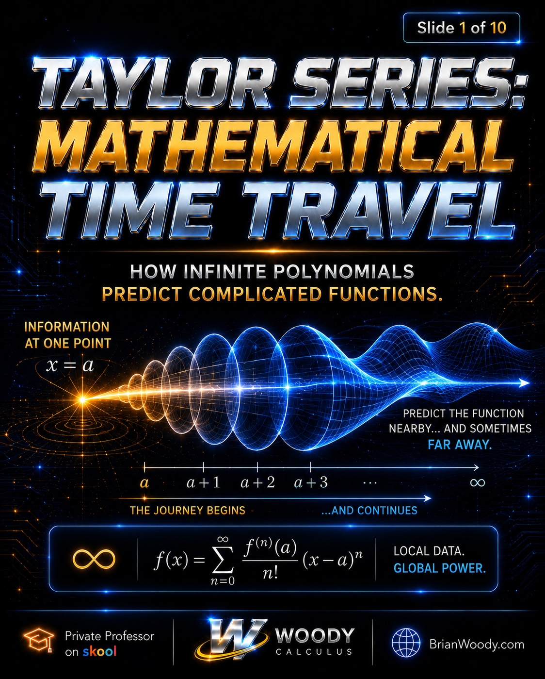
Ever wonder how calculators can approximate values like \(e^x\), \(\sin x\), or \(\ln(1+x)\) so quickly?
The answer is one of the most powerful ideas in Calculus 2: the Taylor Series.
A Taylor Series takes information from one point and uses it to build a polynomial model of a function. In other words, Taylor Series allow us to replace complicated functions with polynomial patterns we can compute, manipulate, approximate, and understand.
This is why Taylor Series are not just another topic in Calculus II. They are a bridge between Calculus 2, Calculus 3, Differential Equations, physics, finance, engineering, numerical analysis, and advanced mathematical modeling.
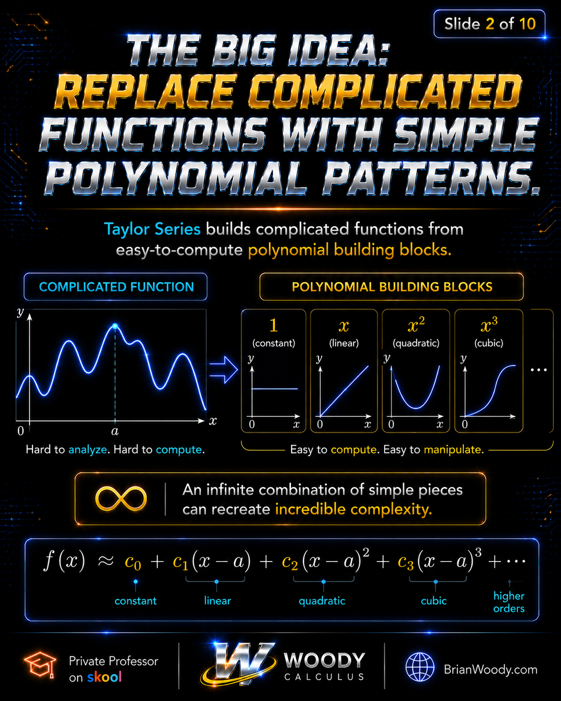
The Big Idea: Replace Complicated Functions with Polynomial Patterns
Polynomials are some of the easiest functions in mathematics to compute, differentiate, integrate, graph, and approximate. A function like
\[
f(x) = c_0 + c_1(x-a) + c_2(x-a)^2 + c_3(x-a)^3 + \cdots
\]
is built from simple pieces: constants, linear terms, quadratic terms, cubic terms, and higher powers.
The Taylor Series idea is that many complicated functions can be represented, at least locally, by an infinite polynomial centered at a chosen point \(x=a\).
Instead of trying to analyze the entire function all at once, we ask a simpler question:
What polynomial behaves like this function near one point?
That question is the beginning of Taylor Series.
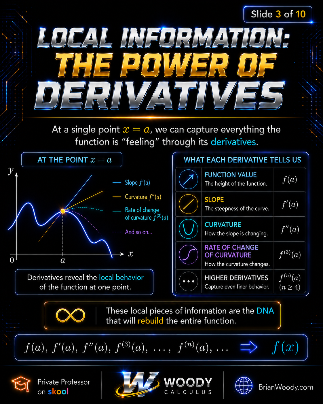
Derivatives Are the DNA of a Function
At a single point \(x=a\), a function carries an incredible amount of information.
The value \(f(a)\) tells us the height of the function.
The first derivative \(f^{\prime}(a)\) tells us the slope.
The second derivative \(f^{\prime\prime}(a)\) tells us curvature.
The third derivative \(f^{(3)}(a)\) tells us how the curvature is changing.
Higher derivatives capture finer and finer behavior.
This is the deeper reason Taylor Series are so powerful. A Taylor Series uses derivative information at one point as the raw material for building a polynomial model of the function.
In this sense, derivatives act like the local DNA of the function. They tell the polynomial how to grow.
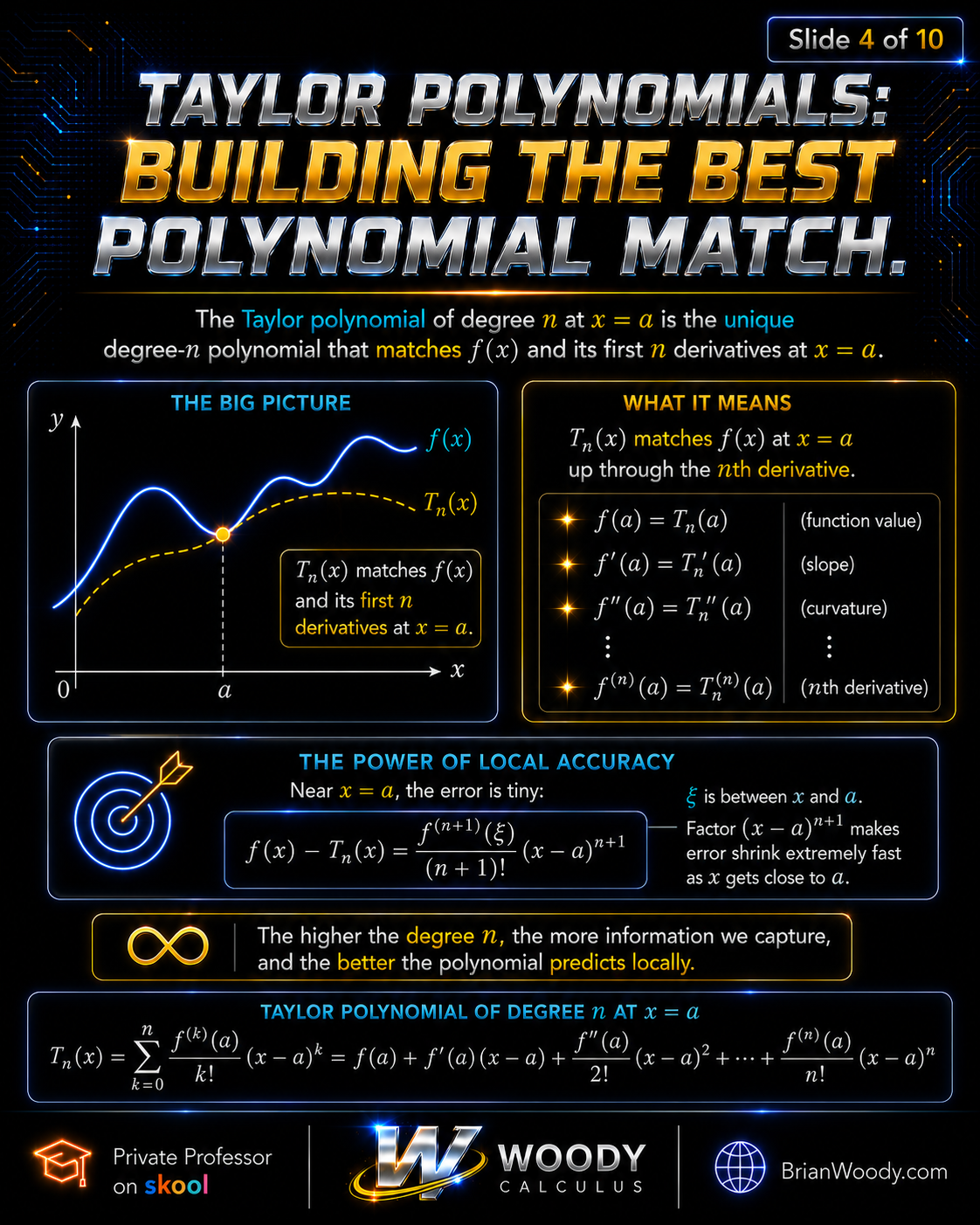
Taylor Polynomials: Building the Best Local Polynomial Match
The Taylor polynomial of degree \(n\) centered at \(x=a\) is the polynomial that matches the function and its first \(n\) derivatives at \(x=a\).
The formula is
\[
T_n(x)=\sum_{k=0}^{n}\frac{f^{(k)}(a)}{k!}(x-a)^k.
\]
Expanded, this becomes
\[
T_n(x)=f(a)+f^{\prime}(a)(x-a)+\frac{f^{\prime\prime}(a)}{2!}(x-a)^2+\cdots+\frac{f^{(n)}(a)}{n!}(x-a)^n.
\]
This polynomial is not random. It is designed so that
\[
T_n(a)=f(a),
\]
\[
T_n^{\prime}(a)=f^{\prime}(a),
\]
\[
T_n^{\prime\prime}(a)=f^{\prime\prime}(a),
\]
and so on, up through the \(n\)th derivative.
That is why Taylor polynomials are so accurate near the center. They are forced to agree with the original function at the point where they are built.
Better Approximations with More Terms
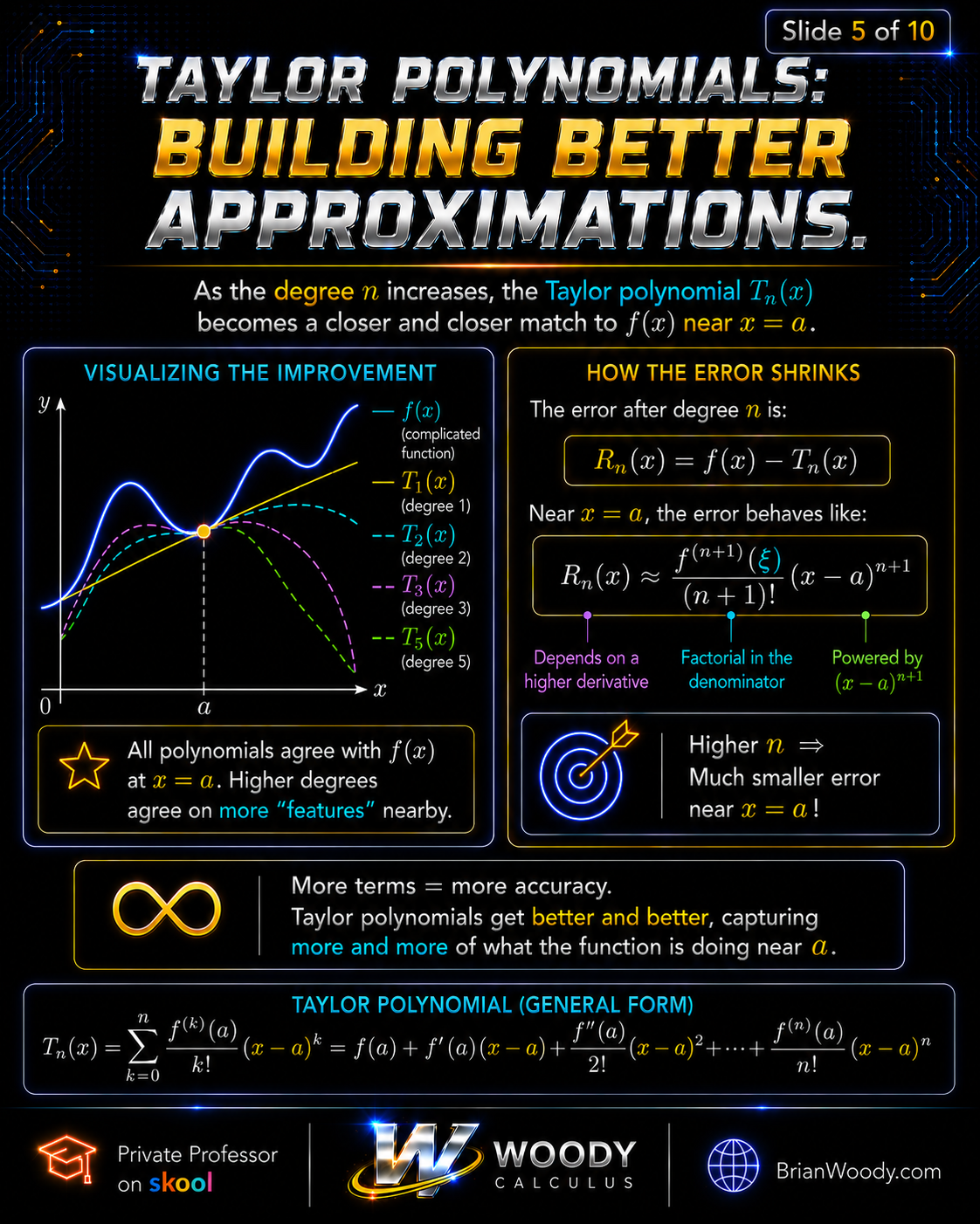
As the degree \(n\) increases, the Taylor polynomial usually becomes a better approximation near \(x=a\).
The first-degree Taylor polynomial captures the function value and slope.
The second-degree Taylor polynomial captures curvature.
The third-degree Taylor polynomial captures how curvature changes.
Higher-degree Taylor polynomials capture more features of the function near the center.
This is where the visual intuition becomes important. Each additional term adds another layer of information. More derivative data usually means a closer local match.
The error after degree \(n\) is often written as
\[
R_n(x)=f(x)-T_n(x).
\]
Near \(x=a\), the error is controlled by a higher derivative and a power of \((x-a)\). This is why Taylor polynomials tend to be extremely accurate close to the center.
The Taylor Series: Infinite Potential
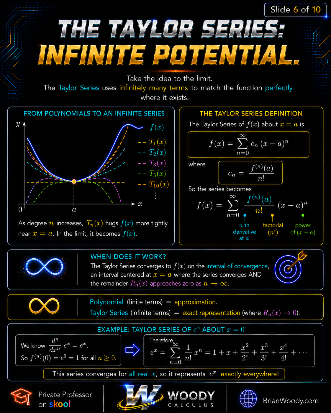
A Taylor polynomial has finitely many terms. A Taylor Series takes the idea to the limit by using infinitely many terms.
The Taylor Series of \(f(x)\) centered at \(x=a\) is
\[
f(x)=\sum_{n=0}^{\infty}\frac{f^{(n)}(a)}{n!}(x-a)^n,
\]
when the series converges to the function.
This condition matters. A Taylor Series is not automatically equal to the original function everywhere. We must consider convergence, the interval of convergence, and whether the remainder term approaches zero.
When it works, though, the result is extraordinary. A complicated function becomes an infinite polynomial.
Example: The Maclaurin Series for \(e^x\)
When \(a=0\), a Taylor Series is called a Maclaurin Series.
For \(f(x)=e^x\), every derivative is still \(e^x\). At \(x=0\), every derivative equals 1.
So the Maclaurin Series for \(e^x\) is
\[
e^x=\sum_{n=0}^{\infty}\frac{x^n}{n!}
=1+x+\frac{x^2}{2!}+\frac{x^3}{3!}+\frac{x^4}{4!}+\cdots.
\]
This series converges for every real number \(x\), which means it represents \(e^x\) everywhere.
Taylor Series Can Be Centered Anywhere
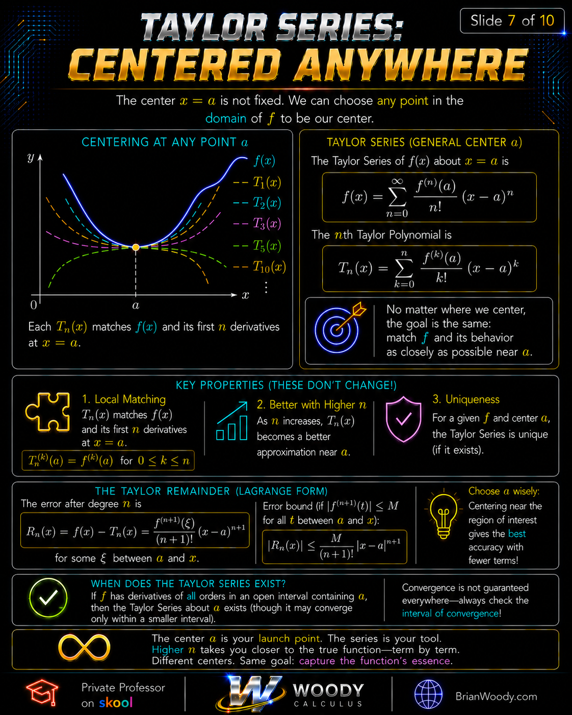
The center does not have to be \(0\). We can center a Taylor Series at any point \(x=a\) where the function has the required derivatives.
The general Taylor Series centered at \(a\) is
\[
\sum_{n=0}^{\infty}\frac{f^{(n)}(a)}{n!}(x-a)^n.
\]
The choice of center matters. If we want a strong approximation near a particular input value, we usually center the Taylor Series near that region.
This is one of the most practical lessons for Calculus 2 students: do not just memorize the formula. Understand what the center is doing.
The center \(a\) is the launch point. The polynomial grows outward from there.
Essential Maclaurin Series Examples
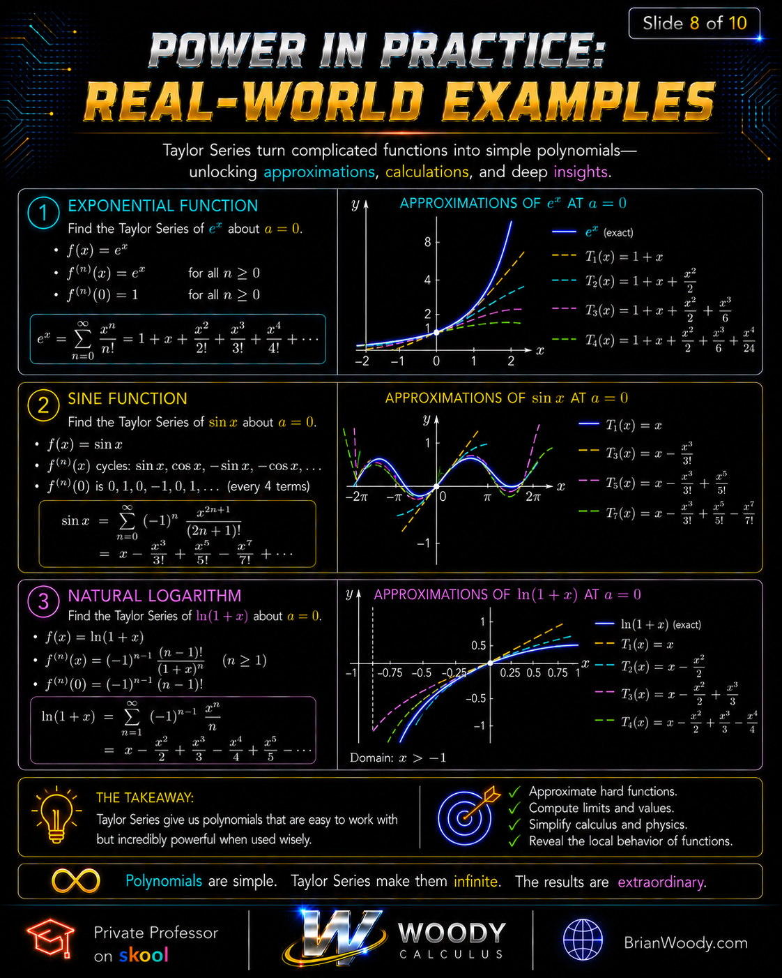
Three of the most important Maclaurin Series in Calculus 2 are the series for \(e^x\), \(\sin x\), and \(\ln(1+x)\).
The Maclaurin Series for \(e^x\)
\[
e^x=1+x+\frac{x^2}{2!}+\frac{x^3}{3!}+\frac{x^4}{4!}+\cdots
\]
This series is one of the most important patterns in all of calculus because it appears in growth models, Differential Equations, probability, complex numbers, physics, and finance.
The Maclaurin Series for \(\sin x\)
\[
\sin x=x-\frac{x^3}{3!}+\frac{x^5}{5!}-\frac{x^7}{7!}+\cdots
\]
The sine series only uses odd powers, and the signs alternate. This pattern comes from the derivative cycle of sine and cosine.
The Maclaurin Series for \(\ln(1+x)\)
\[
\ln(1+x)=x-\frac{x^2}{2}+\frac{x^3}{3}-\frac{x^4}{4}+\frac{x^5}{5}-\cdots
\]
This series is valid on its interval of convergence and is a beautiful example of how a logarithmic function can be rewritten as an infinite polynomial.
Real-World Applications of Taylor Series
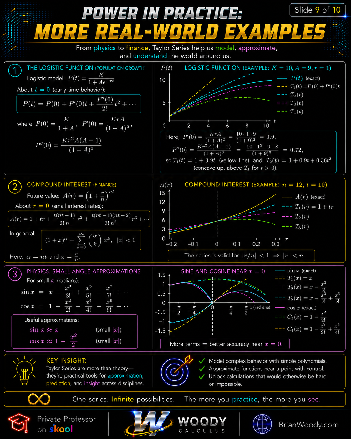
Taylor Series are not just theoretical. They are practical tools used throughout mathematics, science, engineering, economics, and data modeling.
Logistic Growth and Population Models
The logistic function
\[
P(t)=\frac{K}{1+Ae^{-rt}}
\]
appears in population growth, biology, epidemiology, and modeling systems with limiting capacity.
Near \(t=0\), Taylor polynomials can approximate early-time behavior:
\[
P(t)\approx P(0)+P^{\prime}(0)t+\frac{P^{\prime\prime}(0)}{2!}t^2+\cdots.
\]
This is especially useful when studying local behavior before long-term saturation dominates the model.
Compound Interest and Finance
Compound interest involves expressions like
\[
A(r)=\left(1+\frac{r}{n}\right)^{nt}.
\]
Taylor Series help approximate how the value changes for small interest rates. This connects Calculus 2 to finance, exponential growth, and long-term modeling.
Physics and Small-Angle Approximations
In physics, one of the most important uses of Taylor Series is small-angle approximation.
For small \(x\), measured in radians,
\[
\sin x\approx x
\]
and
\[
\cos x\approx 1-\frac{x^2}{2}.
\]
These approximations are used in pendulum motion, waves, oscillations, mechanics, and Differential Equations.
This is the power of Taylor Series: they allow us to replace difficult functions with simpler polynomial models that are easier to use.
Why Taylor Series Matter in Calculus 2
Taylor Series are one of the moments where Calculus 2 becomes truly powerful.
At first, students often see Taylor Series as another formula to memorize. But the real point is much deeper.
Taylor Series show that complicated functions can be understood through local patterns. The function value, slope, curvature, and higher derivatives at one point can generate a polynomial model that reveals the structure of the function.
That is a major shift in mathematical thinking.
Instead of seeing \(e^x\), \(\sin x\), and \(\ln(1+x)\) as separate formulas, we begin to see them as patterns generated by derivatives.
This is exactly the kind of pattern recognition that advanced mathematics demands.
The Woody Calculus Method: Train the Pattern Until It Becomes Automatic
At Woody Calculus, I do not teach Taylor Series as disconnected memorization.
I teach students to memorize the right structures through deliberate, efficient mathematical training.
The goal is not passive memorization. The goal is automatic mastery.
That means rewriting perfect solutions, saying the steps out loud, and repeating correct mathematical patterns until the mechanics become automatic.
When the mechanics become automatic, the mind has room to see the deeper structure. That is when visualization, intuition, and genuine understanding begin to grow.
This matters especially in Calculus II, where students must recognize series patterns quickly:
- When to use a Taylor Series
- How to find derivatives efficiently
- How to identify a Maclaurin Series
- How to use known series patterns
- How to determine the interval of convergence
- How to estimate error
- How to apply Taylor Series to real-world models
Students do not become strong at Taylor Series by staring at formulas. They become strong by working the patterns until recognition becomes immediate.

Get Help with Taylor Series, Calculus 2, and Advanced Mathematics
If you are taking Calculus 2 and Taylor Series are starting to feel overwhelming, you are not alone.
This topic combines derivatives, infinite series, convergence, approximations, factorials, powers, and algebraic pattern recognition. It is one of the biggest conceptual jumps in Calculus II.
Inside Woody Calculus Private Professor on Skool, students get support with:
- Calculus II
- Calculus III
- Differential Equations
- Linear Algebra
- Abstract Algebra
- Real Analysis
- AP Calculus BC
You can get video courses, live Q&A, chat help, past exams, full written solutions, and structured support for university mathematics.
The Woody Calculus Method works — if you work it.
Join Woody Calculus Private Professor on Skool or visit BrianWoody.com to learn more.
Related Woody Calculus Mathematical Essays
For more visual mathematical essays connecting Calculus II, Calculus III, Differential Equations, Abstract Algebra, and Real Analysis, explore these Woody Calculus blog posts:
- How to Learn Calculus and Advanced Mathematics
- Gabriel’s Horn: Finite Volume and Infinite Surface Area
- Line Integrals and Vector Fields
- Fourier Series
- The Cantor Set
- Galois Theory
- View All Woody Calculus Blog Posts
Universities Supported by Woody Calculus
Woody Calculus supports students at universities across the country with Calculus II, Calculus III, Differential Equations, Linear Algebra, Abstract Algebra, Real Analysis, and advanced mathematics coursework.
- University Calculus Tutor Hub
- Colorado State University Calculus Help
- UCF Calculus Tutor
- Purdue Calculus Tutor
- University of Florida Calculus Tutor
- Georgia Tech Calculus Tutor
- Texas A&M Calculus Tutor
- Penn State Calculus Tutor
- Arizona State Calculus Tutor
- UCLA Calculus Tutor
- UCSD Calculus Tutor
- Michigan State Calculus Tutor
- Virginia Tech Calculus Tutor
- University of Washington Calculus Tutor
- UIUC Calculus Tutor
- Rutgers Calculus Tutor
- University of Maryland Calculus Tutor
- Indiana University Calculus Tutor
- UNC Calculus Tutor
- Auburn Calculus Tutor
- SDSU Calculus Tutor
- UNR Calculus Tutor
Great content!