Two methods.
A very different error.
The trapezoidal rule and Simpson’s rule can start with exactly the same function values and produce surprisingly different answers. In this lesson, you will work one integral both ways, see where the weights come from, and measure how close each estimate gets.
Follow the ten Woody Calculus slides in order, then use the written calculations to practice each step. The extended lesson includes error bounds, a complete practice solution, midpoint and Romberg connections, and a counterexample showing why Simpson’s rule does not always win.
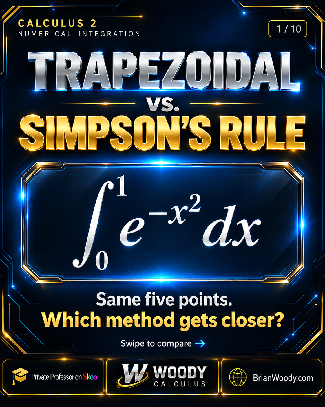
- Trapezoidal T4
- 0.742984
- Simpson S4
- 0.746855
- Benchmark
- 0.746824133
The estimates are rounded for display. Error comparisons below use the unrounded calculations.
Start here
What is the difference between the trapezoidal rule and Simpson’s rule?
The trapezoidal rule joins adjacent sample points with straight lines. Simpson’s rule fits a quadratic through each group of three successive points. Both approximate a definite integral using function values. The standard composite formulas below use equally spaced samples; Simpson’s 1/3 rule also requires an even number of subintervals.
Trapezoidal rule
Use the endpoint heights once and every interior height twice. Multiply the weighted sum by h/2.
- 1
- 2
- 2
- 2
- 1
Any positive integer n · Straight-line approximation
Simpson’s rule
Use endpoint weights 1. Alternate interior weights 4, 2, 4, 2, …, 4. Multiply by h/3.
- 1
- 4
- 2
- 4
- 1
Even positive integer n · Quadratic approximation
Why approximate an integral at all?
Sometimes you have a table of measurements instead of a formula. Sometimes you know the function, but its antiderivative cannot be written with elementary functions. Numerical integration gives you a way to estimate the accumulated quantity in either situation.
Our example, f(x) = e−x², has no elementary antiderivative. It still has a perfectly well-defined definite integral. Because the function is positive on [0, 1], that integral is the area beneath the curve.
These methods belong in your Calculus 2 toolkit alongside the symbolic methods in integration techniques.
If an exam gives you a table, these rules convert the available heights into an estimate of signed area. If it gives you a formula, you first build the table yourself. The workflow is the same: width, nodes, heights, weights, sum, multiplier. Keeping those parts separate prevents most setup errors.
Slide 02 / Build the grid
How do you choose the width and sample points?
We will approximate ∫01 e−x² dx using n = 4 equal subintervals. Here, n counts the spaces between the nodes. Four subintervals require five sample points.
![Divide [0, 1] into four equal subintervals: h = (1 − 0)/4 = 0.25. The five sample points are 0, 0.25, 0.50, 0.75, and 1.](https://k3p6r8v3.delivery.rocketcdn.me/wp-content/uploads/2026/10/Trapezoidal-vs-Simpsons-rule-Slide-2.png)
Subinterval width
Count spaces, then points. The intervals are [0, 0.25], [0.25, 0.50], [0.50, 0.75], and [0.75, 1.00]. There are four spaces and five endpoints. In general, n subintervals give n + 1 nodes.
Include both endpoints. Starting at x = 0.25 omits the first height; treating five nodes as five intervals changes h and produces the wrong weighted sum. Before evaluating the function, check that your last node is exactly b.
Slide 03 / One table for both rules
Evaluate the five heights once.
Now substitute each node into f(x) = e−x². Squaring happens before the minus sign: at x = 0.50, the exponent is −(0.50)² = −0.25.
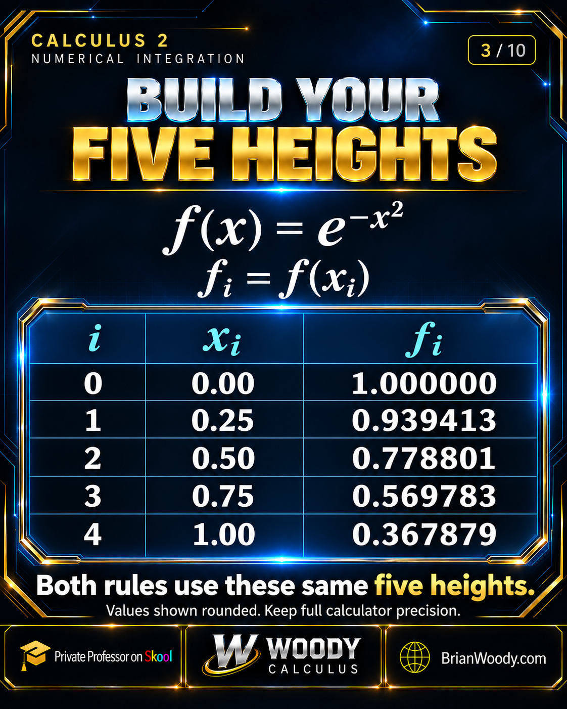
| i | Node xi | Height fi = f(xi) |
|---|---|---|
| 0 | 0.00 | 1.000000 |
| 1 | 0.25 | 0.939413 |
| 2 | 0.50 | 0.778801 |
| 3 | 0.75 | 0.569783 |
| 4 | 1.00 | 0.367879 |
Keep the calculator’s full precision. The rounded table is for reading. Both final six-decimal estimates agree if you use these printed heights, but the more detailed error comparison later uses unrounded function values.
Calculator input: keep the exponent together.
Enter exp(-(0.50)^2), or the equivalent exponential key sequence on your calculator. This is e−0.25. It is different from squaring e−0.50. Store the function values at full precision if your calculator allows it, and round the final estimates only after adding the weighted terms.
How each rule uses those heights
Trapezoidal rule
Four straight top edges
Simpson’s rule
Two quadratic panels
The cyan graph joins adjacent heights with straight lines. The gold graph uses one quadratic through nodes 0, 1, 2 and another through nodes 2, 3, 4. Both approximations meet every sampled point. Their behavior between the points determines the difference in area.
Slide 04 / Build the trapezoidal rule
Trapezoidal rule formula: why are the weights 1, 2, 2, 2, 1?
For n equal subintervals, write fi = f(a + ih). The general formula is:
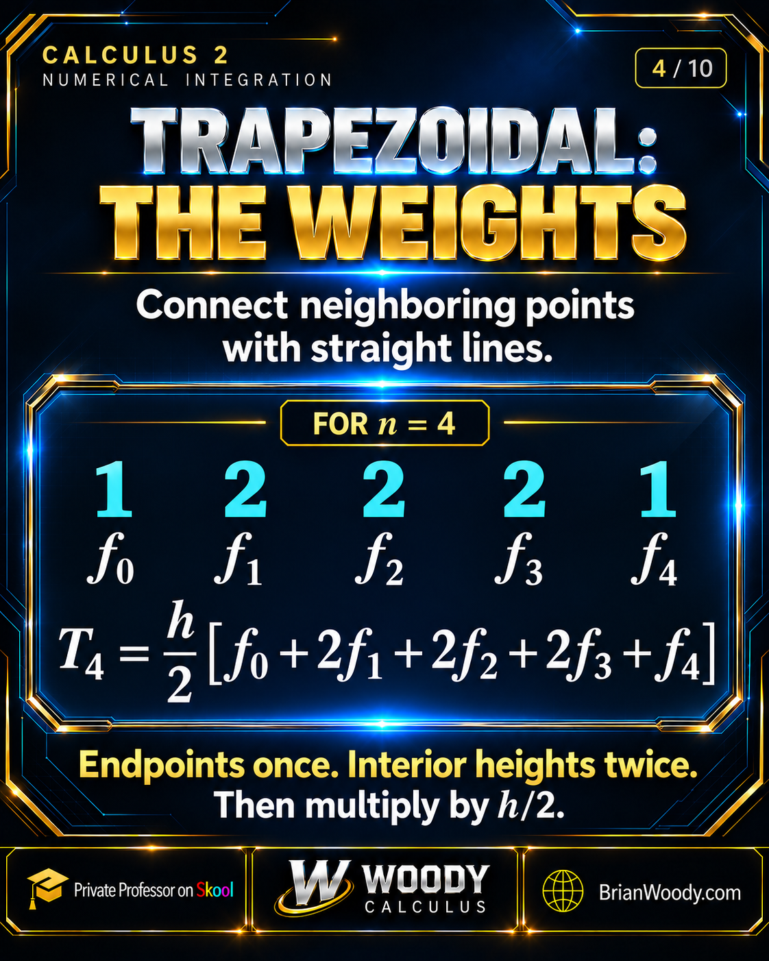
Trapezoidal rule formula
Why are the interior weights 2?
One trapezoid contributes h(fi + fi+1)/2. When you add neighboring trapezoids, each interior height appears in two of them. The first and last heights appear only once. That gives the endpoint weights 1 and the interior weights 2.
= h × fi + fi+12.
The first and last sample heights each belong to one trapezoid. Every interior height is shared by the trapezoid on its left and the trapezoid on its right. That is where the factor 2 comes from; it is a counting consequence of the geometry.
Slide 05 / Work the arithmetic
Calculate the trapezoidal estimate T₄.
Write the weights first, then place the five heights underneath them in the same order. With h = 0.25, the multiplier h/2 is 0.125.
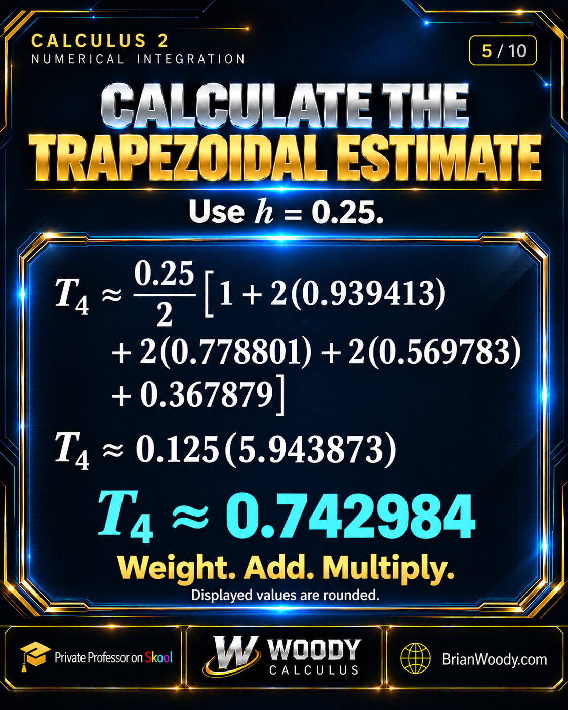
Substitute n = 4 and h = 0.25
T4 ≈ 0.742984
Using full-precision heights: T4 ≈ 0.742984097800.
The structure is simple: width factor, weights, heights, sum. Keep those pieces in that order and you have a repeatable calculation.
Say what you are doing: “I keep the first height. I double each of the three interior heights. I keep the last height. I add the weighted heights. I multiply the sum by 0.125.”
Using the six-decimal heights printed on the slide gives 0.125 × 5.943873 = 0.742984125. Using full-precision heights gives 0.742984097800381…. Both round to 0.742984 at six decimal places. The small difference matters only when you compare more digits or calculate a precise error.
Slide 06 / Build Simpson’s 1/3 rule
Simpson’s rule formula: why 1, 4, 2, 4, 1?
Simpson’s rule groups the subintervals in pairs. Each pair supplies three points for a quadratic fit. That pairing is why n must be even in the standard composite 1/3 rule.
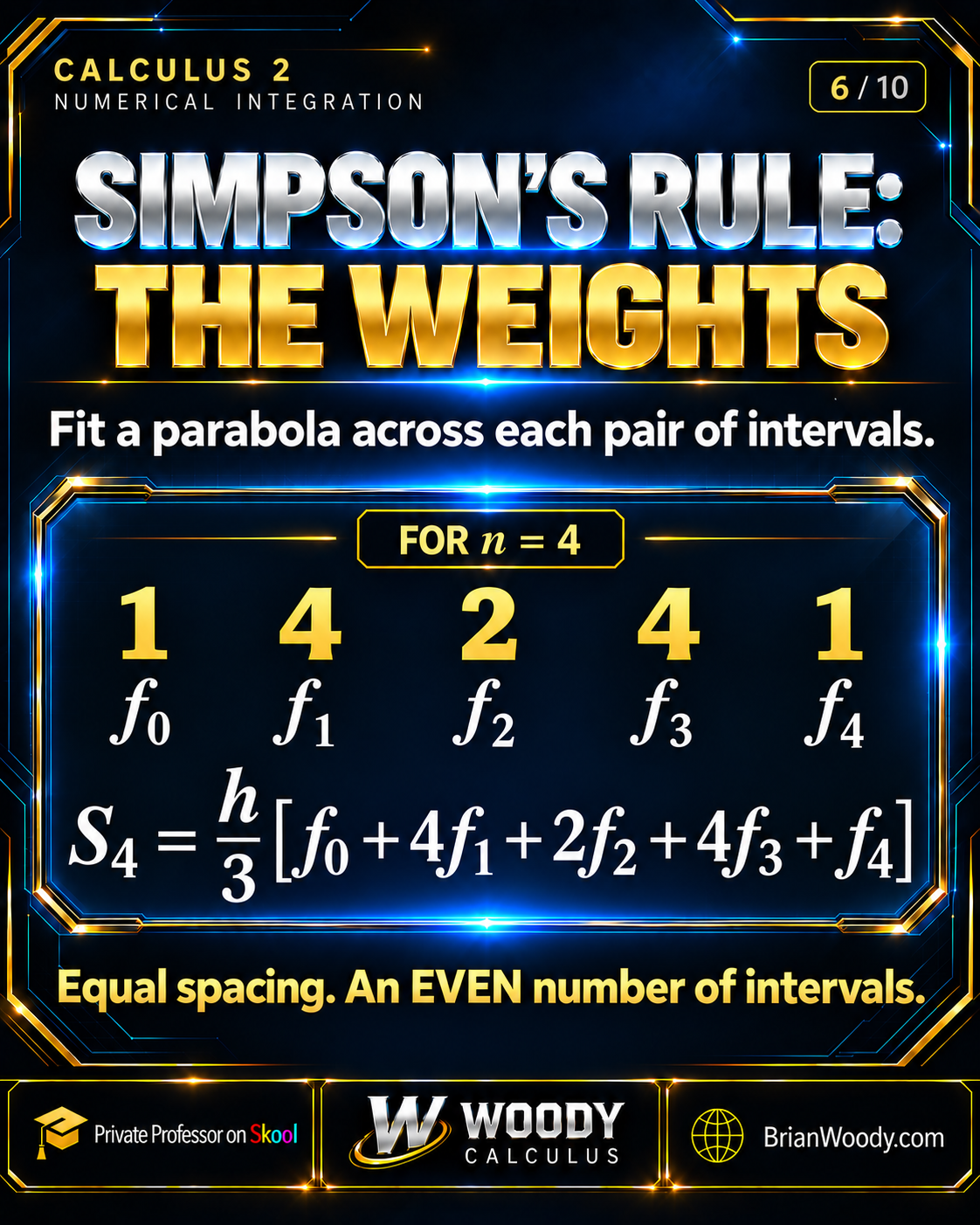
Simpson’s rule formula · n even
Interior odd indices get weight 4. Interior even indices get weight 2. Both endpoints get weight 1.
Where does the 1–4–2–4–1 pattern come from?
Integrating one fitted quadratic across two subintervals gives the panel formula (h/3)(f0 + 4f1 + f2). Our second panel contributes (h/3)(f2 + 4f3 + f4). Add them: the shared height f2 appears twice.
The shared height f2 appears at the end of the first panel and the start of the second, so its combined coefficient is 2. The midpoint heights f1 and f3 each receive weight 4. The outermost heights still receive weight 1.
The multiplier is h/3, where h is the width of one subinterval. A whole quadratic panel has width 2h, but substituting 2h for h in the final formula doubles the estimate incorrectly. Pairing the subintervals is also why the standard composite 1/3 rule requires even n.
Slide 07 / Reuse the heights
Calculate Simpson’s estimate S₄.
The function values have not changed. Replace the trapezoidal weights with 1, 4, 2, 4, 1, and replace h/2 with h/3.
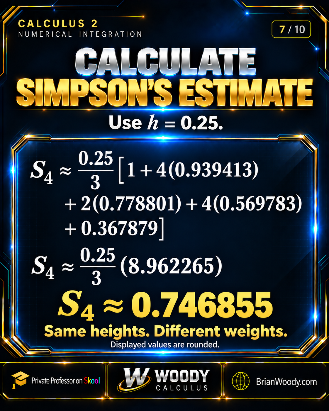
Calculate Simpson’s estimate
S4 ≈ 0.746855
Using full-precision heights: S4 ≈ 0.746855379791.
Keep 0.25/3 exact until the end. Replacing it early with 0.0833 throws away precision before the weighted sum is even multiplied.
Using the displayed six-decimal heights gives 8.962265/12 = 0.74685541666…. The full-precision calculation gives 0.746855379790987…. Both display as 0.746855. Keep the unrounded result available for the next step.
Slide 08 / Measure the error
How accurate are the two estimates?
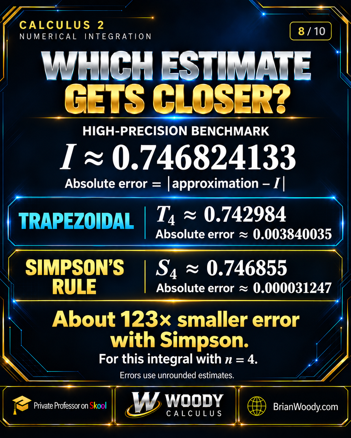
A high-precision benchmark for our integral is I ≈ 0.746824132812427. In special-function notation, its exact value is (√π/2) erf(1). You do not need the error function to apply either rule.
Absolute error measures distance from the true value: |I − approximation|.
Trapezoidal rule T4
- Estimate
- 0.742984
- Absolute error
- 0.003840035
Simpson’s rule S4
- Estimate
- 0.746855
- Absolute error
- 0.000031247
Same five function evaluations. Errors use unrounded estimates.
For this integral with n = 4, Simpson’s rule has about 123 times smaller absolute error.
We did not add more sample points. We changed how the same heights were combined. The trapezoidal estimate is below the benchmark; Simpson’s estimate is slightly above it.
That is the useful comparison: the same data can support different approximation methods with very different errors. The factor 123 belongs to this example. It is not a general guarantee for Simpson’s rule.
Why your subtraction may differ: subtracting the displayed six-decimal estimates from the benchmark introduces their rounding error. The table’s error figures were computed before those estimates were rounded.
Slide 09 / Check before submitting
Five numerical integration mistakes to catch early.
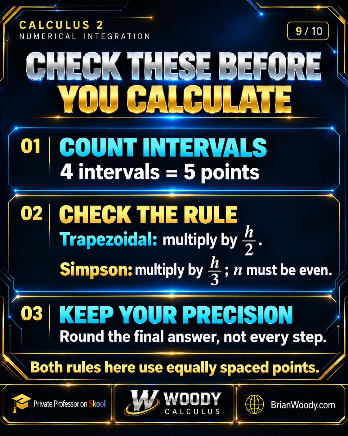
- Counting the points as n. Four subintervals have five nodes. Use the interval count in h = (b − a)/n.
- Using h/2 in Simpson’s rule. Trapezoidal uses h/2; Simpson’s 1/3 rule uses h/3.
- Doubling the endpoint heights. Both rules give the endpoints weight 1.
- Applying the standard Simpson pattern to odd n or uneven spacing. Check the sample spacing and interval count before substituting.
- Rounding midway through the calculation. Keep stored function values and multipliers at full precision; round the reported estimate at the end.
Overestimate or underestimate? The trapezoidal rule overestimates for a function that is concave up throughout the interval and underestimates for one that is concave down throughout. For e−x², the second derivative is (4x² − 2)e−x², which changes sign at x = 1/√2. A single concavity label does not cover [0, 1].
Slide 10 / Try it independently
Your turn: approximate the integral of 1/(1 + x²).
Approximate the integral below with the trapezoidal rule and Simpson’s rule using n = 4. Then compare both estimates with the exact value π/4.
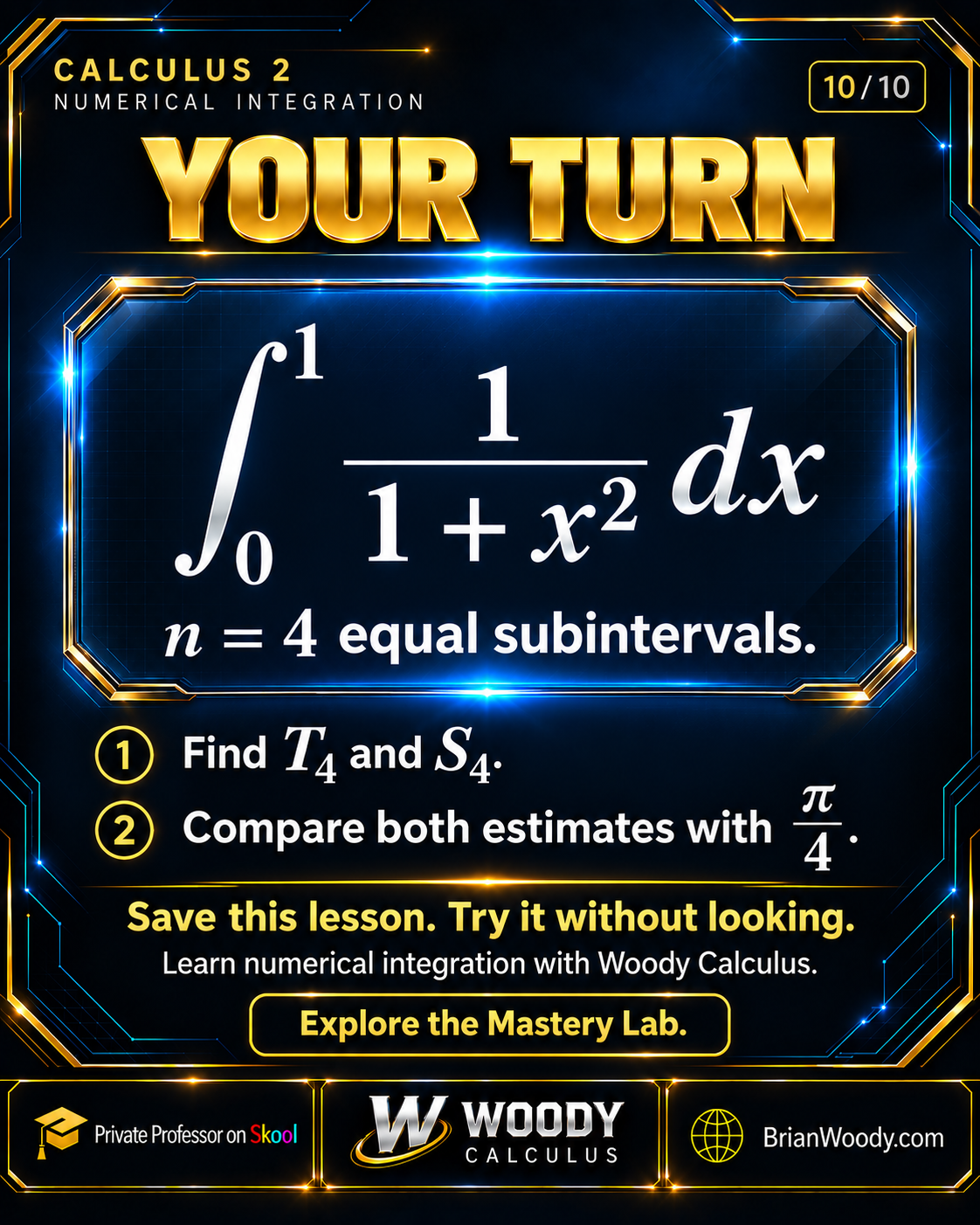
- Find h and list the five nodes.
- Evaluate the five heights.
- Apply each set of weights and its multiplier.
- Compute both absolute errors using unrounded estimates.
Reveal the complete worked solution
1. Width and nodes
Again, h = 1/4. The nodes are 0, 1/4, 1/2, 3/4, and 1.
| x | Exact height | Decimal display |
|---|---|---|
| 0 | 1 | 1.000000 |
| 1/4 | 16/17 | 0.941176 |
| 1/2 | 4/5 | 0.800000 |
| 3/4 | 16/25 | 0.640000 |
| 1 | 1/2 | 0.500000 |
2. Trapezoidal estimate
T4 ≈ 0.782794
3. Simpson’s estimate
S4 ≈ 0.785392
4. Exact integral and errors
An antiderivative is arctan x, so the exact integral is arctan(1) − arctan(0) = π/4 ≈ 0.785398163397.
|π/4 − T4| ≈ 0.002604046
|π/4 − S4| ≈ 0.000006007
Both estimates are below the true value. Simpson’s is much closer for this example. The errors use the exact fractions above, not the displayed six-decimal estimates.
Go further / Guaranteed accuracy
Trapezoidal and Simpson error bounds: how many subintervals do you need?
The actual error compares an approximation with the true integral. An error bound gives a worst-case limit without requiring that true integral first. The standard bounds depend on how large the relevant derivatives can be over the whole interval.
Trapezoidal error bound
If f has a continuous second derivative on [a, b], and |f″(x)| ≤ K2 throughout the interval, then:
Doubling n divides this bound by 4.
Simpson’s error bound
If f has a continuous fourth derivative on [a, b], and |f(4)(x)| ≤ K4 throughout the interval, then:
Use even n. Doubling n divides this bound by 16.
For a fixed interval and sufficiently smooth function, the trapezoidal bound scales like h², while Simpson’s scales like h⁴. Those rates help explain Simpson’s strong performance on many smooth integrals. They do not say that its actual error is always smaller.
Apply the bounds to our Gaussian example.
For f(x) = e−x² on [0, 1], the derivative bounds can be chosen as K2 = 2 and K4 = 12. With n = 4, that gives:
Trapezoidal guarantee
|I − T4| ≤ 212 · 4² = 196
Bound: about 0.0104167.
Actual error: about 0.0038400.
Simpson’s guarantee
|I − S4| ≤ 12180 · 4⁴ = 13840
Bound: about 0.0002604.
Actual error: about 0.0000312.
Both actual errors sit inside their bounds. A bound is a guarantee, not a prediction of the exact error. For related approximation tools, explore alternating-series error and Taylor remainder.
Where do K₂ = 2 and K₄ = 12 come from?
The relevant derivatives are:
f″(x) = (4x² − 2)e−x²
f(4)(x) = (16x⁴ − 48x² + 12)e−x².
On [0, 1], f″ increases from −2 to 2/e, since its derivative is 4x(3 − 2x²)e−x² ≥ 0. Thus the largest absolute value of f″ is 2.
For f(4), check the endpoints and its only interior stationary point, x = √((5 − √10)/2). The values are 12, −20/e ≈ −7.358, and approximately −7.419 at the interior point. The largest absolute value is 12. Both absolute maxima occur at x = 0.
What changes when we double the number of intervals?
Trapezoidal: n = 8
- Estimate T8
- 0.745865615
- Absolute error
- 0.000958518
The error fell by a factor of about 4.01 from n = 4.
Simpson’s: n = 8
- Estimate S8
- 0.746826121
- Absolute error
- 0.000001988
The error fell by a factor of about 15.72 from n = 4.
These observed reductions are close to the factors suggested by the error orders. One calculation illustrates the behavior; it does not prove the general theorem. Ratios were computed with unrounded values.
A useful exactness check
The trapezoidal rule integrates every polynomial of degree at most 1 exactly. Simpson’s rule integrates every polynomial of degree at most 3 exactly. Its quadratic panels also capture the integral of a cubic exactly because the remaining cubic contribution cancels across each symmetric panel.
How do I choose n for a required accuracy?
For a target absolute error no greater than ε, make the appropriate bound no greater than ε.
Trapezoidal: n ≥ √[K2(b − a)3 / (12ε)]
Simpson’s: n ≥ [K4(b − a)5 / (180ε)]1/4
Round up to a positive integer for the trapezoidal rule. For Simpson’s rule, round up to an even positive integer. Your derivative bound must hold everywhere on the interval; sampling a few derivative values does not establish a maximum.
For our example and ε = 10−6: the trapezoidal condition is n ≥ √(1,000,000/6) ≈ 408.248, so choose n = 409 or more. Simpson’s condition is n ≥ (1,000,000/15)1/4 ≈ 16.069, so the smallest allowed even choice is n = 18. These are sufficient counts guaranteed by the bounds, not necessarily the smallest counts that meet the actual error target.
Is Simpson’s rule always more accurate? Here is a counterexample.
No. Consider f(x) = 2 + x⁴ − (9/5)x² on [−1, 1], using n = 2. The three heights are 6/5, 2, and 6/5, and h = 1.
The trapezoidal rule happens to be exact here. Simpson’s has absolute error 4/15. A higher-order error bound is an important advantage under its assumptions; it does not create a universal ranking for every function and every n.
Why is Simpson’s rule exact for cubics if it fits quadratics?
On a panel centered at m with nodes m − h, m, and m + h, let q be the quadratic interpolant to a cubic polynomial p. The difference vanishes at all three nodes, so for some constant A:
This expression is odd in x − m. Its integral over the symmetric interval [m − h, m + h] is zero. Thus p and q have the same integral on the panel, even though they need not be the same function between the nodes. Simpson’s rule integrates q exactly, so it also integrates p exactly. Adding the panels preserves this property.
Go further / Connect the methods
How are midpoint, Simpson’s, and Romberg integration related?
Build Simpson’s estimate from two trapezoidal estimates.
Using the same nested grids, a direct calculation gives this exact identity:
T2 ≈ 0.731370251829 and T4 ≈ 0.742984097800, producing S4 ≈ 0.746855379791.
You can verify the identity by collecting the five function-value coefficients: they become 1, 4, 2, 4, 1 with the h/3 multiplier. For sufficiently smooth functions, this combination cancels the leading second-order term in the trapezoidal error expansion. It is the first Richardson-extrapolation step used in Romberg integration.
Where does the midpoint rule fit?
The midpoint rule samples the center of each subinterval. For four intervals on [0, 1], use 0.125, 0.375, 0.625, and 0.875, with width h = 0.25.
Here M4 is the midpoint estimate; K4 above is a derivative bound. The midpoint estimate is above the true integral, with absolute error about 0.001922999. Its error is roughly half the trapezoidal error in this example.
Combining the four-interval midpoint and trapezoidal data creates the nine-node grid for Simpson’s rule with eight intervals:
Keep the subscripts straight: this combination gives S8, not S4.
Beyond this finite-interval example, the full Gaussian integral is ∫−∞∞ e−x² dx = √π. Infinite limits require an improper-integral setup; the finite-interval rules above cannot simply take h = ∞.
Use the method appropriately
What if the data are unevenly spaced, noisy, or incomplete?
The formulas in the ten-slide lesson assume equally spaced nodes. First inspect the x-values in a supplied table. Equal gaps in the printed columns do not guarantee equal gaps in the actual numbers.
Unequal spacing: add individual trapezoids.
The trapezoidal idea still works when widths differ. Order the nodes so x0 < x1 < … < xn. Give each interval its own width and add its signed area:
Sum over i = 0, 1, …, n − 1.
You cannot apply the usual alternating 1, 4, 2, 4, …, 1 Simpson weights unchanged to arbitrary unequal spacing. Use an appropriate unequal-node quadrature formula, or a method specified by your course.
An odd number of subintervals
The standard composite Simpson’s 1/3 rule requires even n. If you are free to sample the function again, choose an even number of equal subintervals. If you must use a fixed table, follow the assigned method. Combining 1/3 and 3/8 rules can handle some grids, but that is a different formula and should be labeled explicitly.
Measured data and uncertainty
A smaller theoretical discretization error does not remove measurement error from a table. Higher-order interpolation is not automatically the best choice for noisy or poorly resolved data. Check the sample spacing, what the values represent, and whether the smoothness assumptions behind an error guarantee are justified.
Infinite endpoints or singularities
These finite-interval error formulas do not apply unchanged across a singularity or an infinite endpoint. Begin with the limit definitions in the improper integrals lesson; a numerical treatment then needs an appropriate truncation, transformation, or specialized method.
Practice with Woody
Write the pattern. Say what you are doing. Then use it.
Take a complete, correct worked solution and rewrite it 3–5 times. As you write, say what you are doing out loud, clearly and confidently. Keep the narration tied to the line you are writing:
“I divide the interval length by four. I evaluate the five heights. For the trapezoidal rule, I use one, two, two, two, one. I multiply the weighted sum by h over two.”
For Simpson’s rule, rehearse its own pattern: “One, four, two, four, one. Multiply by h over three.” Think of naming notes while practicing a guitar scale: the spoken words follow the action.
Then put the model away and attempt the practice problem independently. Check the weights, the multiplier, and the arithmetic. Come back to the technique in a later session. The 3–5 count is my teaching guideline; your independent work shows what you can use.
If you lose track of a step, bring that exact line to the Lab. Read more about the routine in the Woody Calculus study guide.
Learn Calculus 2 with the Woody Calculus Mastery Lab.
Keep learning with Woody
Bring your next Calculus 2 problem to the Mastery Lab.
Work with video lessons, complete solutions, and guidance from Woody. Find the relevant method, practice the steps, and ask about the part that is holding you up.
Then $89/month. Course coverage varies. Private one-on-one instruction is separate.
Look inside before you join
Tour the Mastery Lab and see how it works. Watch the tour on YouTube.
Questions students ask
Trapezoidal rule and Simpson’s rule FAQ
When should I use the trapezoidal rule or Simpson’s rule?
Use the method requested in your assignment. For a smooth function sampled at equally spaced points, Simpson’s rule often gives high accuracy with relatively few samples when the number of subintervals is even. The trapezoidal rule is simpler and works with any positive interval count. Its basic panel formula can also accommodate unequal widths, but the single-h formula in this lesson assumes equal spacing.
Why must n be even for Simpson’s rule?
The composite Simpson’s 1/3 rule uses quadratic panels spanning two subintervals each. The intervals must therefore pair up. An odd n needs a different treatment, such as combining compatible rules; do not apply the standard 1–4–2–…–4–1 pattern unchanged.
Does Simpson’s rule always give the smaller error?
No. Simpson’s rule has a higher-order error bound under the required smoothness assumptions, but the actual comparison depends on the function and sample spacing. Our main example favors Simpson’s by about 123 to 1 in absolute error. The counterexample in the error-bounds section shows a function for which the trapezoidal rule is exact and Simpson’s is not.
Is the trapezoidal rule an overestimate or an underestimate?
For a function that is concave up throughout the interval, it is an overestimate; for a function that is concave down throughout, it is an underestimate. If concavity changes, that simple global test does not decide the result. For the e to the minus x squared example here, comparison with the benchmark shows that T₄ is an underestimate.
Why do my error values differ from the ones in this lesson?
The displayed estimates are rounded to six decimal places. The errors were calculated using the unrounded estimates and a high-precision benchmark. Keep full calculator precision through the weighted sum and final multiplication, then round the result you report.
Is Simpson’s rule exact for cubic polynomials?
Yes. With equally spaced samples and an even number of subintervals, the composite Simpson’s 1/3 rule integrates every polynomial of degree at most three exactly, apart from numerical roundoff. This does not mean it integrates every smooth function exactly.
How many points do I need for n subintervals?
You need n + 1 endpoints when both ends of each subinterval are represented in the grid. Four equal subintervals therefore use five points. The midpoint rule instead samples one midpoint per subinterval.
Can I use these rules when I only have a table?
Yes. Use the tabulated function values as the heights. The standard composite trapezoidal and Simpson formulas in this lesson assume equal spacing, and Simpson’s 1/3 rule requires even n. With unequal spacing, add individual trapezoidal areas using their actual widths.
Does an error bound equal the actual error?
No. A valid error bound gives a maximum possible absolute error under its stated derivative assumptions. The actual error may be much smaller. Choosing n from the bound gives a sufficient accuracy guarantee, not necessarily the smallest n that works for a particular function.
Why do we approximate the integral of e^(−x²)?
The function e^(−x²) has no elementary antiderivative. Its integral from 0 to 1 can be written exactly as √π times erf(1), divided by 2, using the error function. Numerical integration supplies a decimal approximation without requiring that special-function notation.
Sources and next steps
Sources, related lessons, and about Woody
The standard composite formulas, exactness properties, and derivative-based error bounds are covered in OpenStax Calculus Volume 2, Section 3.6: Numerical Integration. This lesson’s examples, numerical comparisons, and graphs were calculated for the walkthrough.
This article expands the original ten-slide Woody Calculus Instagram lesson. Every slide appears next to its corresponding written explanation, so you can read, review the image, and practice from the complete calculation.