FLUID EQUATIONS · CALCULUS · THE PROOF CLAIM
Understand the equation. Read the claim precisely.
The incompressible Navier–Stokes equations describe how a fluid’s velocity changes under pressure, viscosity, and external forces while preserving local volume. Understanding the equation is the first step toward understanding a claim about its solutions.
A fluid parcel can accelerate in a steady flow. Viscosity dissipates kinetic energy, but an energy bound alone does not control peak speed. The precise forcing, initial data, domain, and conclusion determine what a proof establishes.
On small screens, swipe long equations sideways. Select a solution heading to reveal its worked answer.
Written and developed by Brian M. Woody, founder of Woody Calculus and former university mathematics lecturer with more than 25 years of teaching experience.
Published · Updated · News sources checked .
Did OpenAI solve Navier–Stokes? Where things stand
Skip to the equations and worked examples
Source check: September 10, 2026. OpenAI announced a proof claim on September 8 and released a paper and Lean materials. It identifies its results with Clay alternatives C/D and says it does not intend to claim the Millennium Prize. Read OpenAI’s announcement.
The paper states a whole-space construction for every positive viscosity: the fluid starts at rest, the force is smooth and compactly supported in space and time, energy remains bounded before time 1, and peak speed has an infinite limsup there. Theorem 1.1 gives the construction; Corollary 10.6 supplies a periodic counterpart. Read the paper.
Clay’s page still displayed “Unsolved” on this source check. That is a dated observation of its listing, not a rejection of the paper. The calculations in this lesson verify our teaching examples; they do not independently verify the research proof. Check Clay’s current listing.
The related work and the dispute over credit
OpenAI’s release contains two distinct claims: forced Navier–Stokes blowup and, in a separate Euler paper, finite-time blowup for unforced three-dimensional Euler flow from smooth, compactly supported initial velocity on \(\mathbb R^3\). Euler has no viscosity term; its unforced result does not establish an unforced Navier–Stokes result.
The related smooth-forcing program appeared before the September 8 announcement: Alpöge and Buckmaster’s Boussinesq and forced-Euler papers, and their porous-medium paper with Matei P. Coiculescu. These papers develop work they credit to Córdoba and Martínez-Zoroa. Tao’s September 7 exposition discusses the program, and OpenAI acknowledges Alpöge and Buckmaster’s priority on forced Euler.
The credit dispute concerns this related blowup research and whether research data contributed to the AI work. Buckmaster describes his concerns and says he does not know whether their data was used. OpenAI says its researchers and agents had not seen Alpöge and Buckmaster’s work before those authors released it publicly, while saying it cannot rule out that de-identified usage data helped improve its models. These are attributed accounts, not findings established by this lesson.
The public Lean repository provides build instructions and a route to independent checking. Availability, successful checking of a formal statement, and expert assessment of its correspondence to the intended problem are separate pieces of evidence.
What are the Navier–Stokes equations?
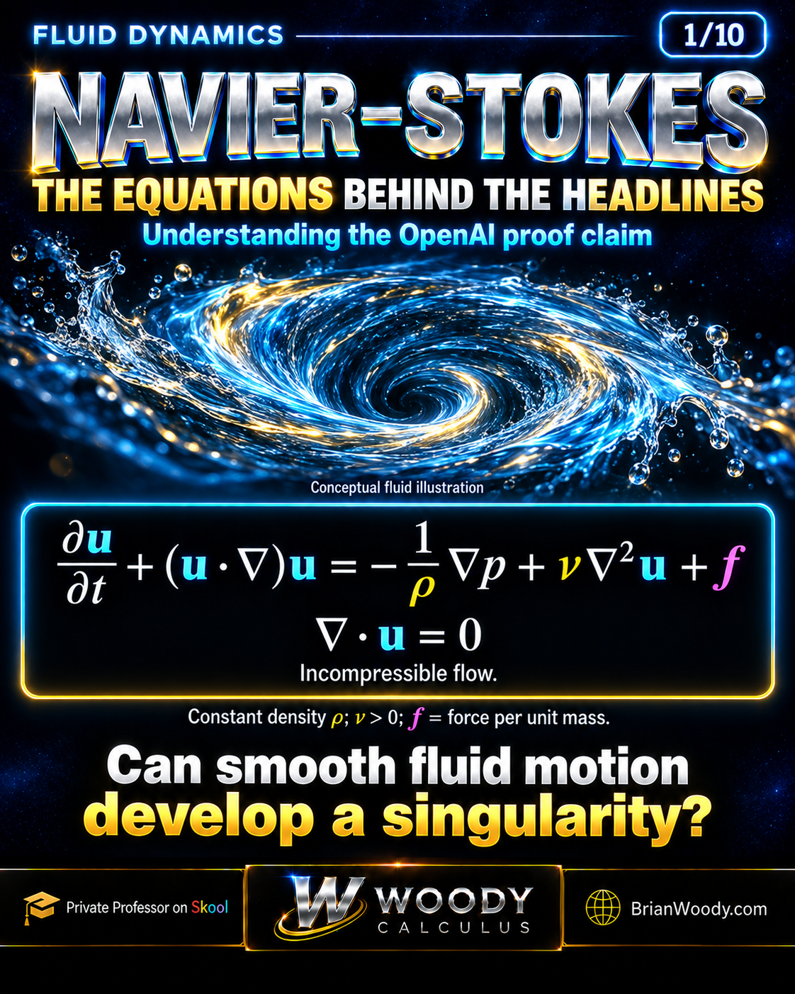
Navier–Stokes is a system of partial differential equations for a fluid’s velocity and pressure. We will study a three-dimensional incompressible Newtonian fluid with constant density and viscosity. “Newtonian” means that viscous stress depends linearly on the rate of deformation; the constant-coefficient model is the one displayed below.
The first equation is Newton’s second law per unit mass. The second is the incompressibility constraint. Together they determine how velocity and pressure must cooperate. An equation alone is not a complete problem: we also need a domain, initial velocity, boundary conditions when there is a boundary, and a specified external force.
Our notation uses physical pressure \(p\). Some mathematical papers divide pressure by density and call the result pressure as well. Setting \(\pi=p/\rho\) changes the pressure term to \(-\nabla\pi\); it does not change the underlying constant-density model.
| Symbol | Meaning | SI units |
|---|---|---|
| \(\mathbf u\) | Velocity vector | m/s |
| \(p\) | Physical pressure | Pa = kg/(m·s²) |
| \(\rho\) | Mass density | kg/m³ |
| \(\nu\) | Kinematic viscosity | m²/s |
| \(\mu=\rho\nu\) | Dynamic viscosity | Pa·s |
| \(\mathbf f\) | External force per unit mass | m/s² |
A quick units check catches many mistakes. \(\nu\Delta\mathbf u\) has units \((\mathrm{m^2/s})(\mathrm{m/s})/\mathrm{m^2}=\mathrm{m/s^2}\). Pressure divided by density and differentiated in space also gives acceleration. A force density measured in newtons per cubic meter would need division by density before it could be used as our \(\mathbf f\).
Velocity fields, pressure, and incompressibility

At a fixed time, a velocity field gives a vector at every location. It is not the track of one particular particle. Write \(\mathbf u=(u_1,u_2,u_3)\); each component may depend on all three spatial coordinates and time. The pressure field assigns one scalar value at each location.
Imagine placing a probe in a river: the probe reports changing velocity at its fixed position. Now release a small floating marker: its path records motion through positions. The first is an Eulerian description; the second is a Lagrangian description. In an unsteady flow, an instantaneous streamline need not coincide with a particle’s path over time.
Zero divergence does not mean zero motion
For a material volume \(V(t)\) moving with a smooth flow, its rate of volume change is the integral of divergence over that volume. Zero divergence therefore preserves local fluid volume. A parcel may stretch in one direction and compress in another while keeping its volume unchanged.
For example, \(\mathbf u=(ax,-ay,0)\) has divergence \(a-a=0\) even though most particles move. By contrast, \(\mathbf u=(ax,ay,az)\) has divergence \(3a\) and is not incompressible when \(a\ne0\). These are kinematic divergence checks, not yet full momentum-equation verifications.
The Divergence Theorem connects this local statement to net flux through a closed surface. Our partial derivatives lesson explains the coordinate derivatives used here.
Read every term before trying to solve anything
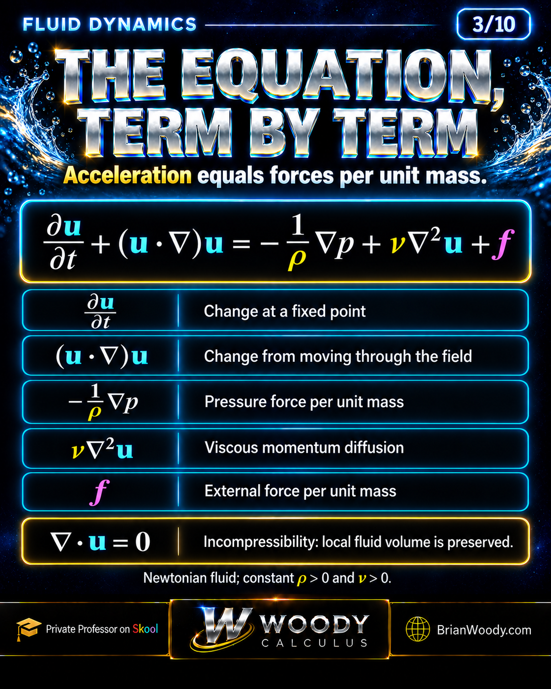
| Term | Mathematical role | Physical interpretation |
|---|---|---|
| \(\partial_t\mathbf u\) | Local time derivative | Change measured at a fixed position. |
| \((\mathbf u\cdot\nabla)\mathbf u\) | Convective derivative | Change experienced while moving through a spatially varying field. |
| \(-\nabla p/\rho\) | Pressure-gradient force per mass | Pressure pushes from higher toward lower pressure. |
| \(\nu\Delta\mathbf u\) | Second spatial derivatives | Viscosity diffuses momentum. |
| \(\mathbf f\) | Specified external acceleration | For example, gravity when it has not been absorbed into pressure. |
The gradient and Laplacian do different jobs
The pressure gradient is a vector built from first derivatives of one scalar field. The vector Laplacian applies the scalar Laplacian separately to each velocity component. The symbol \(\nabla^2\) on the slides means this Laplacian; it is not a componentwise square of velocity.
The negative pressure-gradient direction follows the same geometry as steepest descent. Review gradients and directional derivatives if the sign feels mysterious. A pressure drop along the positive x direction produces a pressure acceleration in the positive x direction.
Why the material derivative makes Navier–Stokes nonlinear
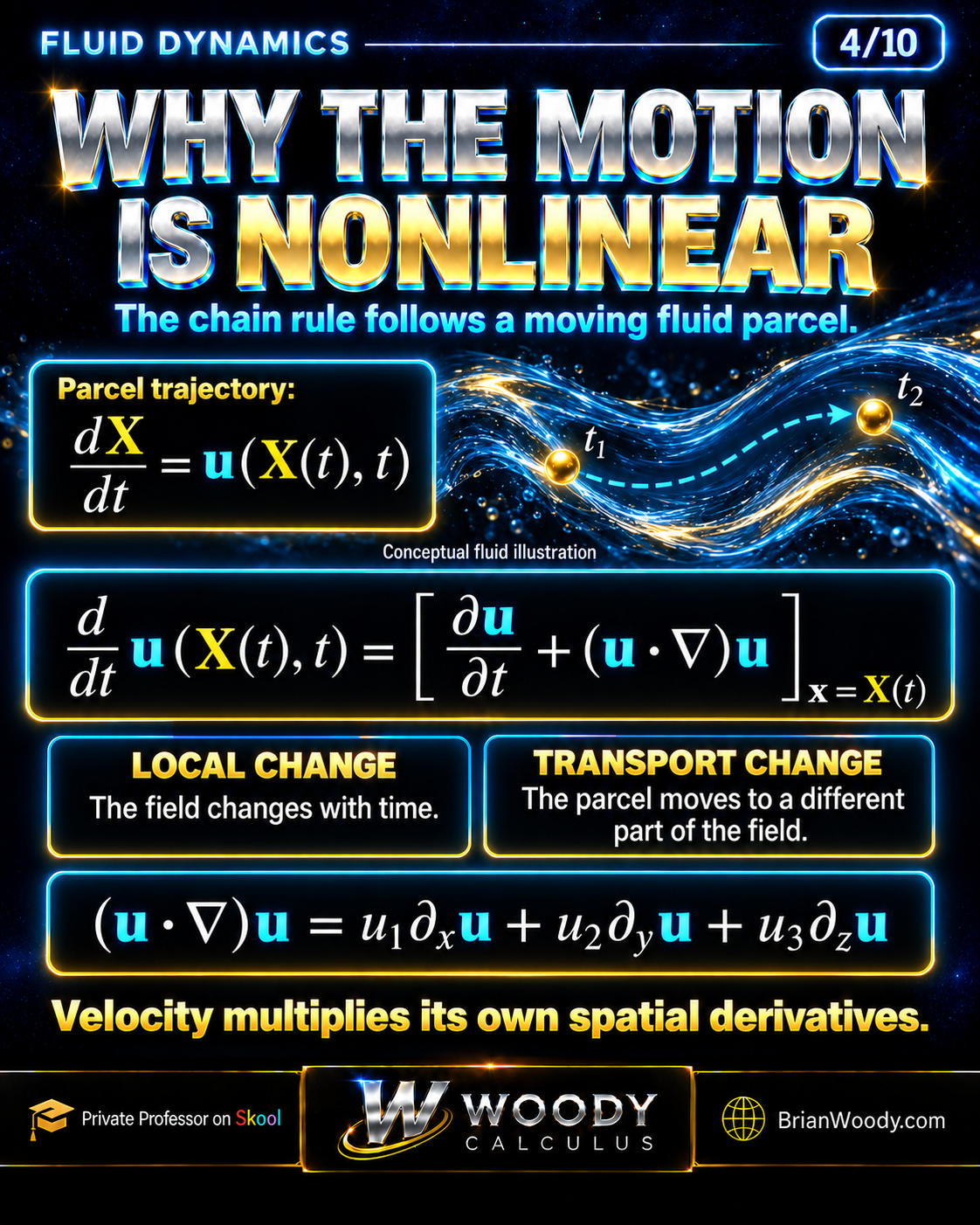
Let \(\mathbf X(t)\) be a fluid parcel’s position. The parcel must move at the velocity assigned by the field where it currently is:
Differentiate one component of the velocity measured along this path. There is a direct time dependence and a contribution from each changing coordinate:
Every expression on the right is evaluated at \((\mathbf X(t),t)\). Substituting the trajectory equation gives:
The field helps choose the path along which the field is differentiated. This is why the transport term is nonlinear. Multiplying a velocity field by a constant multiplies its transport term by the square of that constant, whereas its local time derivative scales only linearly.
A steady flow can still accelerate
Take the time-independent incompressible field \(\mathbf u=(ax,-ay,0)\), with constant \(a\). Its local time derivative is zero, but direct differentiation gives:
A particle can accelerate because it moves into a location where the velocity differs. “Steady” describes the field at fixed locations; it does not say each moving particle has constant velocity. This local example isolates the meaning of convection without claiming the whole-space decay conditions in the Millennium problem.
Vorticity, stretching, and viscous smoothing
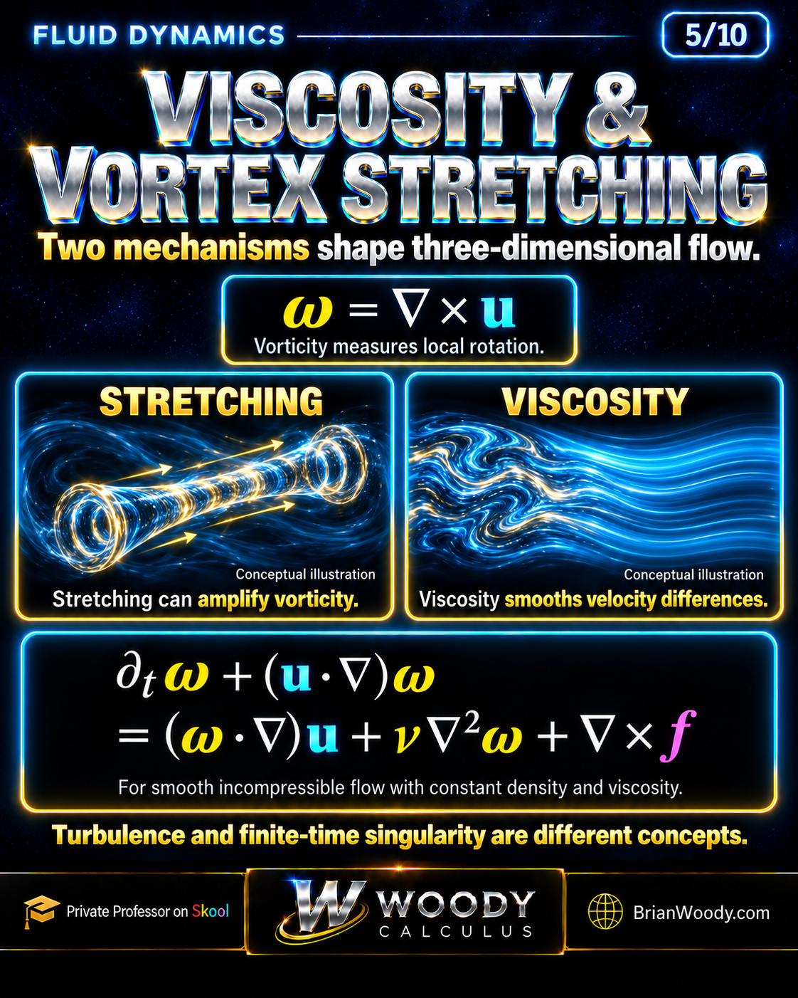
Vorticity is the curl of velocity, \(\vec{\omega}=\nabla\times\mathbf u\). It records local rotation. For rigid rotation, its magnitude is twice the angular speed; a curved particle path alone is not the definition of vorticity.
Take the curl of the momentum equation. For sufficiently smooth fields, curl commutes with time differentiation and the Laplacian. Constant density makes the pressure contribution disappear because the curl of a gradient is zero. The incompressible result is:
The stretching term differentiates velocity in the vorticity direction. Its component along vorticity can amplify or weaken the local spin; other components can change its direction. Viscosity supplies diffusion, while a force with nonzero curl can contribute to rotation.
In planar two-dimensional flow embedded in three dimensions, velocity has no vertical component and is independent of the vertical coordinate. Vorticity points vertically, so \((\vec{\omega}\cdot\nabla)\mathbf u=\mathbf0\). This removes the stretching mechanism in that setting. It does not make every fluid problem easy, but it identifies one structural difference between two and three dimensions.
Turbulence is not a synonym for singularity
Irregular-looking motion can remain mathematically smooth. A finite-time singularity concerns failure of smooth continuation in a specified solution class. Neither a dramatic vortex picture nor a turbulent simulation proves that failure.
Exact solution: verify a decaying periodic shear flow
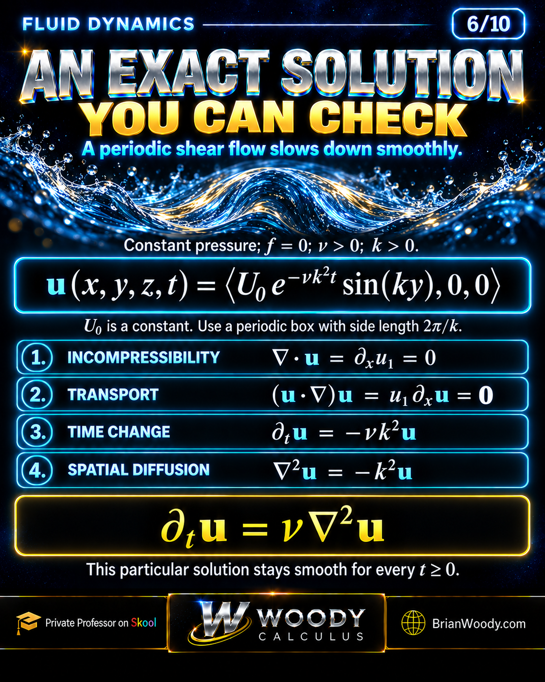
Before discussing a difficult existence problem, verify one solution completely. Let \(U_0\) be a real constant, \(\nu>0\), and \(k>0\). Use a periodic cube with side \(L=2\pi/k\), constant pressure, and zero forcing:
1. Check incompressibility
Only the x-component is nonzero, and it depends on y and t rather than x. Divergence differentiates that component with respect to x:
2. Check the nonlinear term
The velocity points in the x direction, so it transports the field through x derivatives. Those derivatives vanish:
3. Compute the time derivative and Laplacian
The time derivative brings down the exponential decay factor. Two y derivatives of the sine bring down \(-k^2\); the x and z derivatives vanish:
4. Substitute into the complete equation
Both sides agree at every point and time. The initial velocity is \((U_0\sin(ky),0,0)\), and the sine is periodic with the stated side length. This is an exact solution, not an approximate numerical match.
The domain is part of the answer
When U0 is nonzero, this shear is independent of x and z, so its total kinetic energy on all of three-dimensional space would be infinite. The example uses a finite periodic cell. Finding one globally smooth solution also does not prove that every admissible initial velocity has one.
Worked numbers: velocity and energy decay at different rates
Assume \(U_0\ne0\) and let \(A(t)=|U_0|e^{-\nu k^2t}\) be the peak speed of the shear field. Its time constant is \(\tau=1/(\nu k^2)\). After one time constant the peak is \(1/e\) times its initial value.
For \(U_0=2\ \mathrm{m/s}\), \(\nu=0.01\ \mathrm{m^2/s}\), and \(k=2\ \mathrm{m^{-1}}\), the exponent is dimensionless because \(\nu k^2\) has units of inverse seconds. We obtain:
Integrate the energy instead of guessing its rate
Integrate over one periodic cube \([0,L]^3\). Since the average of sine squared over a period is one half:
The square of velocity doubles the exponential rate. Consequently the energy fraction after 25 seconds is \(e^{-2}\approx0.135335\), even though the peak-speed fraction is \(e^{-1}\approx0.367879\).
| Quantity | General half-time | This example |
|---|---|---|
| Peak speed | \(\ln2/(\nu k^2)\) | \(25\ln2\approx17.3287\ \mathrm{s}\) |
| Kinetic energy | \(\ln2/(2\nu k^2)\) | \(12.5\ln2\approx8.66434\ \mathrm{s}\) |
The energy reaches half its initial value in half the time needed for the velocity amplitude to do so. Doubling the wavenumber makes both decay rates four times larger: viscosity damps this shorter spatial wavelength more rapidly.
Two steady channel flows: Couette and Poiseuille
Different boundary conditions lead to different exact solutions. The periodic shear above decays without energy input. A moving wall or an imposed pressure drop can instead sustain steady motion. These channel examples also show why one cannot discuss a fluid equation without its physical setting.
Couette flow: a moving wall drives a linear profile
Place stationary and moving parallel plates at \(y=0\) and \(y=H\), where \(H>0\). Let the upper plate move with velocity \(U\mathbf e_x\). With constant pressure and zero body force:
No slip gives velocity zero at the bottom plate and \(U\mathbf e_x\) at the top. Divergence, local time derivative, and convection are zero. The only nonzero first derivative is \(\partial_yu_1=U/H\), whose second derivative is zero, so \(\Delta\mathbf u=\mathbf0\). The momentum equation is satisfied.
Plane Poiseuille flow: a pressure drop drives a parabola
Now hold both plates fixed at \(y=\pm h\), with \(h>0\). Impose physical pressure \(p=p_0-Gx\), where \(G>0\) is the pressure drop per unit length. Set the body force to zero. Seek a steady field \(\mathbf u=(U(y),0,0)\). The x-momentum balance reduces to:
Integrating twice and imposing \(U(-h)=U(h)=0\) gives:
Verification is immediate: \(U_{yy}=-G/(\rho\nu)\), so pressure acceleration \(G/\rho\) cancels viscous deceleration \(-G/\rho\). The maximum occurs at the centerline, where \(U(0)=Gh^2/(2\rho\nu)\). This is flow between parallel plates, not the cylindrical pipe formula.
Steady motion still dissipates energy
The channel walls or imposed pressure drop supply energy. The periodic energy identity with no boundary-work term cannot be applied unchanged to these driven channels. In Couette flow, a zero Laplacian does not mean zero velocity gradient or zero viscous dissipation.
Pressure enforces the incompressibility constraint
Pressure is not generally an arbitrary extra function that can be selected after choosing velocity. Take the divergence of the momentum equation for a smooth incompressible flow. The time and viscous terms have zero divergence. Expanding the remaining velocity derivatives gives:
This is a Poisson equation for pressure, with boundary or periodic conditions still to be specified. It illustrates how pressure responds to the velocity field so that the evolution remains divergence-free. Adding a function of time alone to pressure leaves its spatial gradient unchanged.
Complete the steady acceleration example
Return to \(\mathbf u=(ax,-ay,0)\), with constant \(a\ne0\). Its Laplacian is zero and its convective acceleration is \((a^2x,a^2y,0)\). With no body force, choose:
Then \(-\nabla p/\rho=(a^2x,a^2y,0)\), exactly the acceleration required. The pressure Laplacian is \(-2\rho a^2\), matching the Poisson formula. This verifies the momentum equation as well as incompressibility. The field is a local exact example, not admissible finite-energy whole-space data for the Millennium problem.
Derive the kinetic-energy balance
Take a smooth solution on a periodic cell, or on whole space with sufficient decay and integrability to justify the following operations. Density and viscosity are constant. Dot the momentum equation with \(\rho\mathbf u\) and integrate over the domain \(\Omega\).
The local derivative gives \(dE/dt\). Incompressibility turns the convection contribution into a divergence, whose integral vanishes under these boundary assumptions. The pressure term also becomes a vanishing boundary contribution. Integrating the viscous term by parts gives a negative sum of squared velocity derivatives.
The first term is dissipation; the second is the power supplied by the body force. Without forcing, kinetic energy is nonincreasing in this setting. With forcing, energy need not decrease: the sign and size of the work term matter.
Check the identity against the shear solution
For the sinusoidal shear, integrating cosine squared gives the same factor of one half from averaging over a period as sine squared, hence \(\int|\nabla\mathbf u|^2=k^2\int|\mathbf u|^2\). The energy law becomes:
That independently reproduces the exponent derived by direct integration. It is a useful habit: calculate a quantity in two ways and check that the interpretations agree.
This is an equality for the smooth solutions under the stated assumptions. Weak-solution theories require their own hypotheses and may provide an energy inequality instead. An energy estimate alone does not automatically supply every derivative bound needed for smooth continuation.
How can energy stay bounded while peak speed grows?
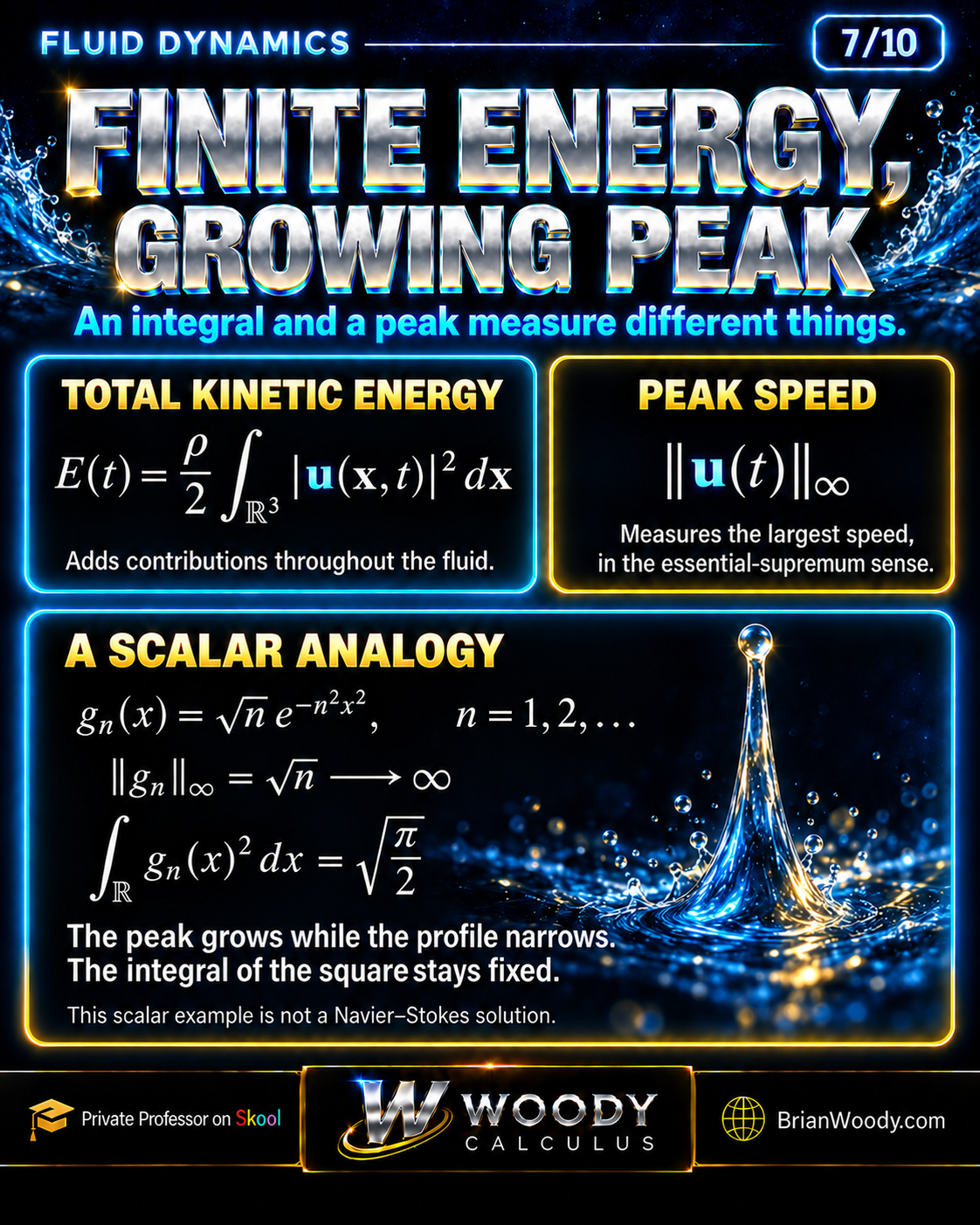
Energy aggregates squared speed over volume. A peak measures how large speed becomes locally. A growing amplitude can occupy a shrinking region, so the integral and the peak need not grow together. The following exact scalar example makes the distinction calculable.
The exponential is at most one and equals one at the origin. Therefore \(\|g_n\|_\infty=\sqrt n\to\infty\). For the integral of the square, use \(s=nx\), so \(dx=ds/n\):
Thus \(\|g_n\|_2^2=\sqrt{\pi/2}\) and \(\|g_n\|_2=(\pi/2)^{1/4}\) stay fixed. The squared norm and the norm are different numbers; both are bounded here. This example shows that no bound on this L² norm alone controls the L-infinity norm on the real line.
Maximum versus essential supremum
The L-infinity norm is an essential supremum: changing a function on a set of measure zero does not change it. For these continuous Gaussians, it agrees with the attained maximum. A general function on an unbounded domain need not attain its supremum. Our supremum and infimum lesson develops the distinction between a least upper bound and a maximum.
An analogy establishes only what it proves
The Gaussian sequence is one-dimensional and scalar. It is not a fluid solution and does not demonstrate Navier–Stokes blowup. It demonstrates the gap between two kinds of bounds, which is why controlling total energy need not finish a regularity proof.
Reynolds number: compare inertia with viscosity
Choose a characteristic speed \(U>0\) and length \(L>0\). Use the advective time \(L/U\), pressure scale \(\rho U^2\), and dimensionless variables \(\mathbf x=L\mathbf x^*\), \(t=(L/U)t^*\), \(\mathbf u=U\mathbf u^*\). Dividing the momentum equation by \(U^2/L\) gives:
Here \(\mathbf f^*=(L/U^2)\mathbf f\). Reynolds number is dimensionless. On the chosen scales, it compares convective inertia with viscous diffusion; the coefficient of the dimensionless Laplacian is its reciprocal.
For a hypothetical fluid with \(\nu=10^{-6}\ \mathrm{m^2/s}\), characteristic speed \(U=0.5\ \mathrm{m/s}\), and length \(L=0.02\ \mathrm m\):
That number does not prove turbulence or singularity formation. Transition behavior depends on geometry, disturbances, and how the characteristic scales are defined. In particular, a threshold quoted for one pipe configuration is not a universal threshold for all fluid flows.
What exactly does the Millennium problem ask?
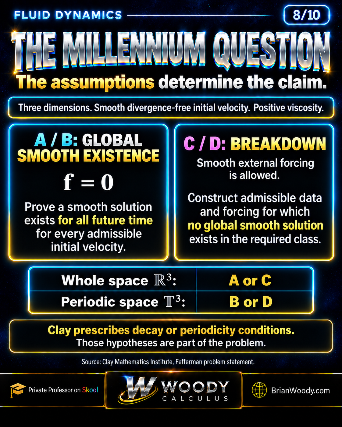
A PDE problem specifies more than a differential expression. Initial regularity, divergence, decay, forcing, spatial domain, and the required solution class all matter. The official Fefferman statement offers four alternatives:
| Alternative | Spatial setting | Task |
|---|---|---|
| A | \(\mathbb R^3\) | Global smooth existence for every admissible initial velocity, with zero forcing. |
| B | Periodic three-dimensional space | The corresponding unforced global smooth-existence statement. |
| C | \(\mathbb R^3\) | An admissible breakdown example allowing suitable smooth forcing, in the required bounded-energy smooth class. |
| D | Periodic three-dimensional space | An admissible breakdown example allowing suitable smooth periodic forcing. |
A forcing term therefore does not automatically place a result outside the official question. Conversely, a forced counterexample is not, by itself, a counterexample with the force set to zero. Preserve the quantifiers: “for every admissible initial velocity” is much stronger than exhibiting one well-behaved example.
Local existence, global existence, and smoothness
Local existence gives a solution for some initial time interval. Global existence extends it to all future times in the stated class. Smoothness asks for the required differentiability, and uniqueness asks whether the same data can produce more than one solution in that class. A weak solution satisfies an integrated formulation and need not have all classical derivatives.
A finite-time singularity refers to failure of smooth continuation at a finite endpoint. Blowup of a particular norm can certify such failure under the relevant framework, but “bounded energy and unbounded peak” is the reported behavior of this construction, not a universal definition for every differential equation.
This is the same logical discipline used in our existence and uniqueness lesson: identify the hypotheses, the domain, and the conclusion before invoking a theorem. The partial differential equation is much harder, but those distinctions remain essential.
Read the announced blowup statement precisely
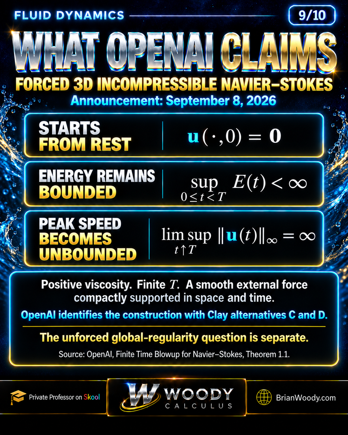
The slide records the announced construction using a generic finite time \(T\). In the paper the endpoint is normalized to \(1\). Its peak conclusion uses a limsup, not a claim that the norm approaches infinity along every possible sequence of times.
This says that arbitrarily large peak values occur arbitrarily close to the endpoint from below. It is stronger than a single large numerical value and more specific than an evocative picture. The force’s smoothness through the relevant time is also crucial: a singular input would change the question being answered.
When comparing sources, preserve their pressure conventions and domains. The whole-space construction and its periodic counterpart are distinct results. The paper and formalization repository are the appropriate starting points for checking exactly which statements are being claimed.
What this lesson verifies
The worked solutions and calculations here can be checked directly. They explain the concepts needed to read the announcement. They are not a substitute for auditing the research proof, its formal statement, or its dependencies.
A six-step checklist for reading a Navier–Stokes claim
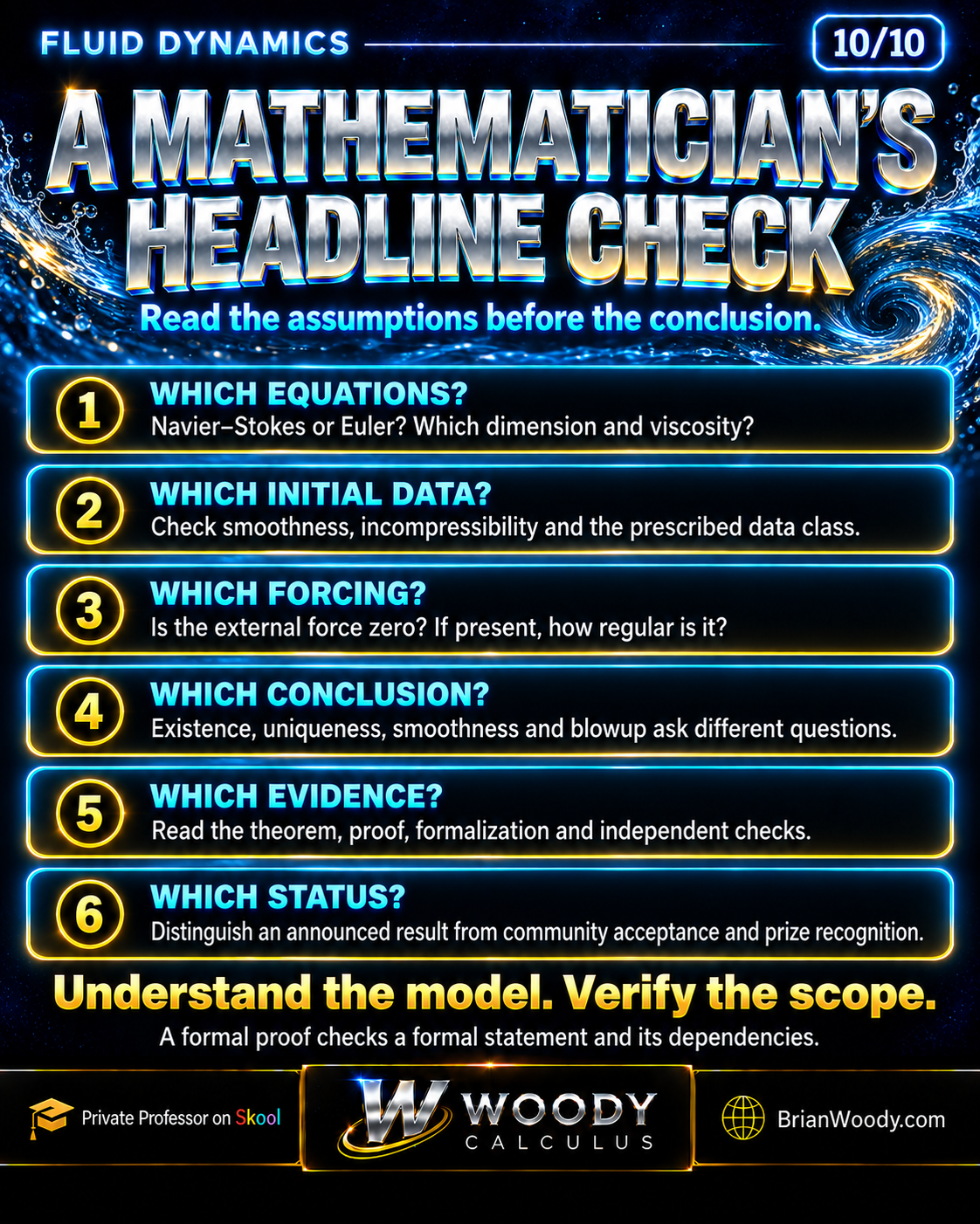
Use the same process for a research headline, a textbook solution, or a numerical experiment. A correct calculation answers only the question whose assumptions it actually meets.
-
Identify the equation and domain
Write the velocity and pressure conventions, density, viscosity, spatial domain, and boundary conditions before interpreting the claim.
-
Check the initial data
Check smoothness, the divergence-free constraint, and the required decay or periodicity of the initial velocity.
-
Inspect the forcing
Determine whether the force is zero or prescribed, and whether it satisfies every required smoothness, support, and time assumption.
-
Read the conclusion and quantifiers
Distinguish one example from every admissible datum, finite time from all time, and energy bounds from smoothness or peak-speed bounds.
-
Examine the evidence
Read the theorem and its proof or formal statement, compare them with the intended problem, and identify the checks that have actually been performed.
-
Report the status accurately
Separate the announced result, independent mathematical assessment, and official recognition; attach a date and primary sources to status claims.
Eight common mistakes to avoid
Zero divergence is not zero velocity
Divergence measures local expansion, not speed. Stretching and compression can balance while the fluid moves.
Steady does not mean zero acceleration
The local time derivative may vanish while the convective derivative remains nonzero.
A divergence check is not a complete solution check
Verify the momentum equation, initial data, forcing, and boundary conditions as well.
The energy integral is not the maximum speed
An integral can stay bounded while peaks concentrate. A squared norm is also distinct from the norm itself.
A forced problem is not an unforced problem
Use the force specified in the statement. Smooth forcing is permitted in Clay alternatives C/D, but cannot simply be removed from a construction.
A simulation is not a proof of a singularity
Numerics are valuable evidence, but finite resolution, discretization, and error control must be distinguished from a continuum theorem.
One smooth example is not an all-data theorem
The periodic shear is globally smooth. That establishes one family, not every admissible three-dimensional flow.
A formalization needs a precise target
A checked formal theorem establishes its encoded statement under its foundations and dependencies. Its correspondence to the intended mathematical claim must also be assessed.
Twelve practice problems with worked solutions
Try each question before opening its solution. The first eleven test calculations and interpretations; the last tests the logical scope of a theorem.
1. Check the units
Pressure \(p\) is measured in pascals, density \(\rho\) in kilograms per cubic metre, velocity in metres per second, and kinematic viscosity \(\nu\) in square metres per second. Check the units of \(-\nabla p/\rho\) and \(\nu\Delta\mathbf u\). What units must \(\mathbf f\) have?
Solution 1: Check the units
A pressure gradient has units \(\mathrm{kg\,m^{-2}\,s^{-2}}\), so division by density gives \(\mathrm{m\,s^{-2}}\). Taking two spatial derivatives of velocity gives \(\mathrm{m^{-1}\,s^{-1}}\); multiplying by \(\nu\) again gives \(\mathrm{m\,s^{-2}}\). Both are accelerations, so \(\mathbf f\) must have units of metres per second squared, equivalently newtons per kilogram: it is force per unit mass.
2. Steady flow can accelerate
In dimensionless variables, \(\mathbf u(x,y,z)=\langle x,-y,0\rangle\) is steady. Calculate its divergence and material acceleration. Evaluate the acceleration at \((1,2,0)\).
Solution 2: Steady flow can accelerate
The divergence is \(1-1=0\), and steadiness gives \(\partial_t\mathbf u=\mathbf0\). However, \((\mathbf u\cdot\nabla)\mathbf u=x\langle1,0,0\rangle-y\langle0,-1,0\rangle=\langle x,y,0\rangle\), so the acceleration at \((1,2,0)\) is \(\langle1,2,0\rangle\). A particle can accelerate while moving through a spatially varying field that is unchanged in time. This is a local calculation; the field does not have finite energy on all of three-dimensional space.
3. Find a shear-flow decay time
A periodic shear has amplitude \(U_0e^{-\nu k^2t}\), with \(U_0=3\,\mathrm{m/s}\), \(\nu=0.02\,\mathrm{m^2/s}\), and \(k=5\,\mathrm{m^{-1}}\). Find its amplitude time constant and amplitude at \(t=2\,\mathrm s\).
Solution 3: Find a shear-flow decay time
The decay rate is \(\nu k^2=(0.02)(25)=0.5\,\mathrm{s^{-1}}\), so the time constant is \(\tau=1/(\nu k^2)=2\,\mathrm s\). At two seconds the exponent is \(-1\), giving amplitude \(3/e\,\mathrm{m/s}\approx1.104\,\mathrm{m/s}\). One time constant reduces the amplitude to \(1/e\) of its initial value.
4. Compare amplitude and energy half-lives
A decaying periodic shear has amplitude time constant \(25\,\mathrm s\). Find the time for its amplitude to halve and the time for its total kinetic energy to halve.
Solution 4: Compare amplitude and energy half-lives
The amplitude ratio is \(e^{-t/25}\), so setting it to \(1/2\) gives \(t=25\ln2\,\mathrm s\approx17.33\,\mathrm s\). Energy is proportional to amplitude squared, making its ratio \(e^{-2t/25}\). Its half-life is therefore \((25/2)\ln2\,\mathrm s\approx8.664\,\mathrm s\), half the amplitude half-life.
5. Evaluate Couette flow
A Couette channel has stationary lower wall, height \(H=0.02\,\mathrm m\), and upper-wall speed \(U=0.3\,\mathrm{m/s}\). For \(\mathbf u=\langle Uy/H,0,0\rangle\), find the midpoint velocity and vorticity.
Solution 5: Evaluate Couette flow
At the midpoint \(y=H/2\), the velocity is \(\langle U/2,0,0\rangle=\langle0.15,0,0\rangle\,\mathrm{m/s}\). The only nonzero vorticity component is \(\omega_z=\partial_xu_2-\partial_yu_1=-U/H=-15\,\mathrm{s^{-1}}\), giving \(\vec{\omega}=\langle0,0,-15\rangle\,\mathrm{s^{-1}}\). Its sign is negative because the positive horizontal velocity increases with height.
6. Evaluate pressure-driven channel flow
For plane Poiseuille flow between walls \(y=\pm h\), take \(h=0.01\,\mathrm m\), \(\rho=1000\,\mathrm{kg/m^3}\), \(\nu=10^{-6}\,\mathrm{m^2/s}\), and \(p=p_0-Gx\) with \(G=2\,\mathrm{Pa/m}\). Find the centerline speed and flow direction.
Solution 6: Evaluate pressure-driven channel flow
At \(y=0\), the speed is:
The flow is in the positive \(x\) direction, toward decreasing pressure, and its velocity vanishes at both walls. The pressure acceleration \(G/\rho\) balances the viscous term \(-G/\rho\); the pressure drop maintains this steady flow.
7. Separate a norm from its square
For \(g_9(x)=3e^{-81x^2}\) on the real line, find its supremum norm, squared \(L^2\) norm, and \(L^2\) norm.
Solution 7: Separate a norm from its square
The maximum occurs at \(x=0\), so \(\|g_9\|_\infty=3\). The Gaussian integral gives \(\|g_9\|_2^2=\int_{\mathbb R}9e^{-162x^2}\,dx=\sqrt{\pi/2}\). Taking the square root once more gives \(\|g_9\|_2=(\pi/2)^{1/4}\); the integral of the square is the squared norm, not the norm itself.
8. Use the energy balance
In consistent nondimensional units on a periodic domain, let \(\rho=2\), \(\nu=1/2\), \(\int_\Omega|\nabla\mathbf u|^2\,dV=3\), and \(\int_\Omega\mathbf f\cdot\mathbf u\,dV=1\). Find \(dE/dt\) and decide whether energy is increasing.
Solution 8: Use the energy balance
The energy balance gives \(dE/dt=-\rho\nu\int|\nabla\mathbf u|^2+\rho\int\mathbf f\cdot\mathbf u=-(2)(1/2)(3)+(2)(1)=-1\). The force contributes positive power, but the viscous loss is larger. Total energy is decreasing at that instant even though the flow is forced.
9. Interpret the Reynolds number
For characteristic speed \(U=0.5\,\mathrm{m/s}\), length \(L=0.02\,\mathrm m\), and viscosity \(\nu=10^{-6}\,\mathrm{m^2/s}\), calculate the Reynolds number. Does that number alone prove turbulence or finite-time blowup?
Solution 9: Interpret the Reynolds number
The Reynolds number is \(\mathrm{Re}=UL/\nu=(0.5)(0.02)/10^{-6}=10000\). Inertial effects are important relative to viscosity at these characteristic scales, but transition also depends on geometry, disturbances, and boundary conditions. This value proves neither turbulence nor finite-time singularity formation.
10. Find a vorticity source
In dimensionless variables, the external force per unit mass is \(\mathbf f(x,y,z)=\langle-y,x,0\rangle\). Calculate its contribution to the vorticity equation.
Solution 10: Find a vorticity source
The contribution is \(\nabla\times\mathbf f=\langle0,0,2\rangle\), because its third component is \(\partial_x(x)-\partial_y(-y)=1-(-1)=2\). Thus this force can directly generate vorticity. The forcing term in the vorticity equation is the curl of the force, not the force itself.
11. Check the initial-data constraint
Is the smooth initial velocity \(\mathbf u_0(x,y,z)=\langle x,y,z\rangle\) divergence-free? Explain whether smoothness alone makes it valid incompressible initial data.
Solution 11: Check the initial-data constraint
Its divergence is \(\partial_x(x)+\partial_y(y)+\partial_z(z)=1+1+1=3\), so it is not divergence-free. Smoothness alone does not satisfy the incompressibility constraint. A candidate initial velocity must meet every assumption, including the specified divergence, domain, boundary, and decay requirements.
12. Read the quantifiers and forcing
(a) Does one globally smooth periodic shear establish global smooth existence for every admissible initial velocity? (b) Does a blowup construction with nonzero force automatically disprove the corresponding zero-force statement?
Solution 12: Read the quantifiers and forcing
(a) No: one verified solution establishes a particular case, whereas an all-data theorem has a universal quantifier. (b) No: nonzero forcing changes the assumptions. A forced construction can address the prescribed C/D alternatives only if it satisfies all their data, regularity, and domain requirements; it does not automatically settle the unforced question.
Navier–Stokes glossary
- Velocity field
- A vector-valued function assigning fluid velocity to each position and time.
- Pressure
- A scalar field whose gradient contributes a force per unit volume; dividing by density gives acceleration.
- Incompressibility
- For a smooth velocity field, the zero-divergence constraint that preserves local material volume.
- Material derivative
- The rate of change of a field measured while following a moving fluid parcel.
- Convective acceleration
- The velocity change caused by moving through a spatially varying velocity field.
- Kinematic viscosity
- Dynamic viscosity divided by density; the positive coefficient of velocity diffusion in this model.
- Laplacian
- The sum of second spatial derivatives; for a vector field it is applied to each component.
- Vorticity
- The curl of velocity, describing local rotational motion.
- Vortex stretching
- The change in vorticity produced by velocity variation along the vorticity direction.
- Kinetic energy
- One half of density times the spatial integral of squared speed.
- Essential supremum
- The least upper bound after disregarding values on sets of measure zero.
- Reynolds number
- The dimensionless ratio UL/nu comparing inertial and viscous effects at chosen characteristic scales.
- Body force
- A force acting through the fluid volume; the force symbol in this lesson is expressed per unit mass.
- Boundary condition
- A condition imposed where the fluid domain meets its boundary, such as a specified wall velocity.
- No-slip condition
- The condition that fluid velocity at a solid wall matches the wall velocity.
- Weak solution
- A solution defined through an integrated formulation that can make sense without all classical derivatives.
- Finite-time blowup
- Unbounded growth of a specified quantity at a finite endpoint, preventing continuation in an appropriate solution class.
- Formal proof
- A derivation expressed in a formal system and checked against its rules and dependencies.
Frequently asked questions
What do the Navier–Stokes equations describe?
They describe the evolution of fluid velocity and pressure. In the constant-density incompressible model, acceleration balances the pressure-gradient force, viscous diffusion, and external forcing, while velocity has zero divergence.
Has OpenAI’s announcement settled the unforced Navier–Stokes question?
The announcement concerns a construction with smooth forcing. A forced construction does not, by itself, settle the corresponding question with zero force. The dated status section links the original statement and current sources.
Why is Navier–Stokes nonlinear?
The convective term multiplies velocity by spatial derivatives of velocity. The fluid motion determines the path along which the velocity field changes.
What does incompressible mean?
In this smooth constant-density model, incompressible means the velocity field has zero divergence and preserves local material volume. It does not mean the velocity is zero or spatially constant.
Can a steady flow have acceleration?
Yes. Steady means no change at a fixed location. A moving particle can still accelerate as it enters locations with different velocities, producing a nonzero convective derivative.
Is there an exact solution of Navier–Stokes?
Yes. Many special configurations have exact solutions. This lesson verifies a periodic decaying sine shear, a moving-wall Couette flow, and pressure-driven flow between parallel plates. Such examples do not establish a theorem for all admissible initial data.
What is the difference between dynamic and kinematic viscosity?
Dynamic viscosity measures the proportionality between viscous stress and deformation rate. Kinematic viscosity is dynamic viscosity divided by density and has units of square meters per second.
Does finite kinetic energy prevent infinite peak speed?
An energy bound alone does not control the peak. The Gaussian sequence in this lesson has a fixed integral of its square and an unbounded peak. It illustrates a distinction between norms; it is not a fluid blowup solution.
Is a high Reynolds number proof of turbulence?
No. Reynolds number compares inertial and viscous effects at chosen scales. Transition depends on geometry, disturbances, and boundary conditions, and the number alone does not prove turbulence or finite-time blowup.
Why is the three-dimensional problem difficult?
Three-dimensional vorticity can stretch, the transport term is nonlinear, and controlling energy does not automatically control all derivatives needed for smooth continuation. The coupled pressure constraint and the required data class also matter.
Does a Lean repository automatically certify a research claim?
A repository provides material to inspect and check. A completed formal check concerns its precise encoded statement and dependencies. Assessing its correspondence to the intended problem and reporting independent review are additional tasks.
What should I study before Navier–Stokes?
Start with partial derivatives, the chain rule, vector fields, divergence, gradients, curl, integration by parts, and ordinary differential equations. The related lessons below build those prerequisites.
Primary sources and further reading
- Charles L. Fefferman — Existence and Smoothness of the Navier–Stokes Equation
Official Clay Millennium problem statement; assumptions and alternatives A–D.
- Clay Mathematics Institute — Navier–Stokes Equation
Current official problem page. Status checked September 10, 2026.
- OpenAI — On the Navier–Stokes Millennium Prize Problem
Announcement dated September 8, 2026; claims and attribution are those of the source.
- OpenAI — Finite Time Blowup for Navier–Stokes
Research manuscript. See Theorem 1.1 and the periodic counterpart, Corollary 10.6.
- OpenAI — Finite Time Blowup for the Euler Equation
Separate research manuscript claiming unforced three-dimensional Euler blowup from smooth compactly supported initial velocity.
- Levent Alpöge and Tristan Buckmaster — Blowup for the Boussinesq Equations with Smooth Forcing
Related smooth-forcing construction in the program credited to Córdoba and Martínez-Zoroa.
- Levent Alpöge and Tristan Buckmaster — Forced Euler preprint
Related Euler blowup construction with smooth forcing; distinct from the unforced Euler claim.
- Levent Alpöge, Tristan Buckmaster, and Matei P. Coiculescu — Porous-medium preprint
Related incompressible porous-medium construction extending the Córdoba–Martínez-Zoroa program to uniformly smooth forcing.
- OpenAI — NavierStokesAndEuler
Public Lean formalization repository and build instructions.
- Terence Tao — Finite time blowup with smooth forcing term
September 7, 2026 exposition of the related porous-medium, Boussinesq, and Euler work.
- Tristan Buckmaster — Public statement
First-person account concerning credit and research-data use. Read alongside the announcement and underlying papers.
The historical and status statements above are dated. The derivative checks and worked examples are independently reproducible calculations in this lesson. If a source or official status changes, update the status section, visible review date, and structured data together.